22 Dec 2016
Unless you use the curves directly authored by the animator for your animation clip, the animation compression you use will end up being lossy in nature and some amount of fidelity will be lost (possibly visible to the naked eye or not). To combat the loss of accuracy, three error compensation techniques emerged over the years to help push the memory footprint further down while keeping the visual results acceptable: in-place correction, additive correction, and inverse kinematic correction.
In-place Correction
This technique has already been detailed in Game Programming Gems 7. As such, I won’t go into implementation details unless there is significant interest.
As we have seen previously, our animated bone data is stored in local space which means that any error on a parent bone will propagate to its children. Fundamentally this technique aims to compensate our compression error by applying a small correction to each track to help stop the error propagating in our hierarchy. For example, if we have two parented bones, a small error in the parent bone will offset the child in object space. To account for this and compensate, we can apply a small offset on our child in local space such that the end result in object space is as close to the original animation as possible.
Up Sides
The single most important up side of this technique is that it adds little to no overhead to the runtime decompression. The bulk of the overhead remains entirely on the offline process of compression. We only add overhead on the decompression if we elect to introduce tracks to compensate for the error.
Down Sides
There are four issues with this technique.
Missing Tracks
We can only apply a correction on a particular child bone if it is animated. If it is not animated, adding our correction will end up adding more data to compress and we might end up increasing the memory footprint. If the translation track is not animated, our correction will be partial in that with rotation alone we will not be able to match the exact object space position to reach in order to mirror the original clip.
Noise
Adding a correction for every key frame will tend to yield noisy tracks. Each key frame will end up with a micro-correction which in turn will need somewhat higher accuracy to keep it reliable. For this reason, tracks with correction in them will tend to compress a bit more poorly.
Compression Overhead
To properly calculate the correction to apply for every bone track, we must calculate the object space transforms of our bones. This adds extra overhead to our compression time. It may or may not end up being a huge deal, your mileage may vary.
Track Ranges
Due to the fact that we add corrections to our animated tracks, it is possible and probable that our track ranges might change as we compress and correct our data. This needs to be properly taken into account, further adding more complexity if range reduction is used.
Additive Correction
Additive correction is very similar to the in-place correction mentioned above. Instead of modifying our track data in-place by incorporating the correction, we can instead store our correction separately as extra additive tracks and combine it during the runtime decompression.
This variation offers a number of interesting trade-offs which are worth considering:
- Our compressed tracks do not change and will not become noisy nor will their range change
- Missing tracks are not an issue since we always add separate additive tracks
- Adding the correction at runtime is very fast and simple
- Additive tracks are compressed separately and can benefit from a different accuracy threshold
However by its nature, the memory overhead will most likely end up being higher than with the in-place variant.
Inverse Kinematic Correction
The last form of error compensation leverages inverse kinematics. The idea is to store extra object space translation tracks for certain high accuracy bones such as feet and hands. Bones that come into contact with things such as the environment tend to make compression inaccuracy very obvious. Using these high accuracy tracks, we run our inverse kinematic algorithm to calculate the desired transforms of a few parent bones to match our desired pose. This will tend to spread the error of our parent bones, making it less obvious while keeping our point of contact fixed and accurate.
Besides allowing our compression to be more aggressive, this technique does not have a lot of up sides. It does have a number of down sides though:
- Extra tracks means extra data to compress and decompress
- Even a simple 2-bone inverse kinematic algorithm will end up slowing down our decompression since we need to calculate object space transforms for our bones involved
- By its very nature, our parent bones will no longer closely match the original clip, only the general feel might remain depending on how far the inverse kinematic correction ends up putting us.
Conclusion
All three forms of error correction can be used with any compression algorithm but they all have a number of important down sides. For this reason, unless you need the compression to be very aggressive, I would advise against using these techniques. If you choose to do so, the first two appear to be the most appropriate due to their reduced runtime overhead. Note that if you really wanted to, all three techniques could be used simultaneously but that would most likely be very extreme.
Note: I profiled with and without error compensation in Unreal Engine 4 and the results were underwhelming, see here.
Up next: Case Studies
Back to table of contents
19 Dec 2016
Signal processing algorithm variants come in many forms but the most common and popular approach is to use Wavelets. Having utilized this method for all character animation clips on all supported platforms for Thief (2014) I have a fair amount to share with you.
Other signal processing algorithm variants include Discrete Cosine Transform, Principal Component Analysis, and Principal Geodesic Analysis.
The latter two variants are commonly used alongside clustering and database approaches which I’ll explore if enough interest is expressed but I’ll be focusing on Wavelets here.
How It Works
At their core implementations that leverage wavelets for compression will be split into four distinct steps:
- Pre-processing
- The wavelet transform
- Quantization
- Entropy coding
The flow of information can be illustrated like this:
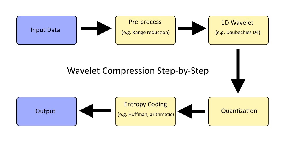
The most important step is, of course, the wavelet function, around which everything is centered. Covering the wavelet function first will help clarify the purpose of every other step.
Aside from quantization all of the steps involved are effectively lossless and only suffer from minor floating point rounding. By altering how many bits we use for the quantization step we can control how aggressive we want to be with compression.
The decompression is simply the same process of steps performed in reverse order.
Wavelet Basics
We will avoid going too in depth on this topic in this series instead we will focus on discussing the wavelet properties and what they mean for us with respect to character animation and compression in general. A good starting point for the curious would be the Haar wavelet which is the simplest of wavelet functions, however, it’s generally avoided for compression.
By definition wavelet functions are recursive. Each application of the function is referred to as a sub-band and will output an equal number of scale and coefficient values each exactly half the original input size. In turn, we can recursively apply the function on the resulting scale values of the previous sub-band. The end result is a single scale value and N - 1 coefficients where N is the input size.
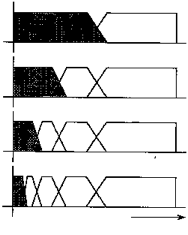
Haar wavelet scale is simply the sum of two input values and the coefficient represents their difference. As far as I know most wavelet functions function similarly which yield coefficients that are as close to zero as possible and exactly zero for a constant input signal.
The reason the Haar wavelet is not suitable for compression because it has a single vanishing moment. This means input data is processed in pairs, each outputting a single scale and a single coefficient. The pairs never overlap which means that if there is a discontinuity in between two pairs it will not be taken into account and yield undesirable artifacts if the coefficients are not accurate. A decent alternative is to use a Daubechies D4 wavelet. This is the function I used on Thief (2014) and it turned out quite decently for our purposes.
The wavelet transform can be entirely lossless by using an integer variant but in practice, an ordinary floating point variant is appropriate since compression is lossy by nature and the rounding will not measurably impact the results.
Since wavelet function decomposes a signal on an orthonormal basis we will be able to achieve the highest compression by considering as much of the signal as possible not unlike principal component analysis. Simply concatenate all tracks together into a single 1D signal. The upside of this is that by considering all data as a whole we can find a single orthonormal basis which will allow us to quantize more aggressively but by having a larger signal to transform the decompression speed will suffer. To keep the process reasonably fast in practice on modern hardware each track would likely be processed independently in a small power of two, such as 16 keys at a time. For Thief (2014), all rotation tracks and translation tracks were aggregated independently up to a maximum segment size of 64 KB. We ran the wavelet transform once for rotation tracks, and once for translation tracks.
Pre-processing
Because wavelet functions are recursive the size of the input data needs to be a power of two. If our size doesn’t match we will need to introduce some form of padding:
- Pad with zeroes
- Repeat the last value
- Mirror the signal
- Loop the signal
- Something even more creative?
Which padding approach you choose is likely to have a fairly minimal impact on compression. Your guess is as good as mine regarding which is best. In practice, it’s best to avoid padding as much as possible by keeping input sizes fairly small and processing the input data in blocks or segments.
The scale of output coefficients is a function of the scale and smoothness of our input values. As such it makes sense to perform range reduction and to normalize our input values.
Quantization
After applying the wavelet transform the number of output values will match the number of input values. No compression has happened yet.
As mentioned previously our output values will be partitioned into sub-bands, and a single scale value somewhat centered around zero — both positive and negative. Each sub-band will end up with a different range of values. Larger sub-bands resulting from the first applications of the wavelet function will be filled with high-frequency information while the smaller sub-bands will comprise the low-frequency information. This is important. It means that a single low-frequency coefficient will impact a larger range of values after performing the inverse wavelet transform. Because of this low-frequency coefficients need higher accuracy than high-frequency coefficients.
To achieve compression we will quantize our coefficients into a reduced number of bits while keeping the single scale value with full precision. Due to the nature of the data, we will perform range reduction per sub-band and normalize our values between [-1.0, 1.0]. We only need to keep the range extent for reconstruction and simply assume that the range is centered around zero. Quantization might not make sense for the lower frequency sub-bands with 1, 2, 4 coefficients due to the extra overhead of the range extent. Once our values are normalized we can quantize them. To choose how many bits to use per coefficient we can simply hard code a high number such as 16 bits, 12 bits, or alternatively experiment with values in an attempt to optimize a solution to meet an error threshold. Quantization could also be performed globally to reduce the range of information overhead instead of per sub-band depending on the number of input values being processed. For example processing 16 keys at a time.
Entropy Coding
In order to be competitive with other techniques, we need to push compression further using entropy coding which is an entirely lossless compression step.
After quantization we obtain a number of integer values all centered around zero and a single scale. The most obvious thing that we can compress now is the fact that we have very few large values. To leverage this we apply a zigzag transform on our data, mapping negative integers to positive unsigned integers such that values closest to zero remain closest to zero. This transforms our data in such a way that we still end up with very few large values which are significant because it means that most of our values represented in memory now have many leading zeroes.
For example suppose we quantize everything onto 16 bit signed integers: -50, 50, 32760. In memory these values are represented with twos complement: 0xFFCE, 0x0032, 0x7FF8. This is not great and how to compress this further is not immediately obvious. If we apply the zigzag transform and map our signed integers into unsigned integers: 100, 99, 65519. In memory these unsigned integers are now represented as: 0x0064, 0x0063, 0xFFEF. An easily predictable pattern emerges with smaller values with a lot of leading zeroes which will compress well.
At this point, a generic entropy coding algorithm is used like zlib, Huffman, or some custom arithmetic coding algorithm. Luke Mamacos gives a decent example of a wavelet arithmetic encoder that takes advantage of leading zeros.
It’s worth noting that if you process a very large input in a single block you will likely end up with lots of padding at the end. This typically ends up as all zero values after the quantization step and it can be beneficial to use run length encoding to compress those before the entropy coding phase.
In The Wild
Signal processing algorithms tend to be the most complex to understand while requiring the most code. This makes maintenance a challenge which is represented by a decreased use in the wild.
While these compression methods can be used competitively if the right entropy coding algorithm is used, they tend to be far too slow to decompress, too complex to implement, and too challenging to maintain for the results that they yield.
Due to its popularity at the time I introduced wavelet compression to Thief (2014) to replace the linear key reduction algorithm used in Unreal 3. Linear key reduction was very hard to tweak properly due to a naive error function it used resulting in a large memory footprint or inaccurate animation clips. The wavelet implementation ended up being faster to compress with and yielded a smaller memory footprint with good accuracy.
Fundamentally the wavelet decomposition allows us to exploit temporal coherence in our animation clip data, but this comes at a price. In order to sample a single keyframe, we must reverse everything. Meaning, if we process 16 keys at a time we must decompress our 16 keys to sample a single one of them (or two if we linearly interpolate as we normally would when sampling our clip). For this reason, wavelet implementations are terribly slow to decompress and speeds end up not being competitive at all which only gets worse as you process a larger input signal. On Thief (2014) full decompression on the Play Station 3 SPU took between 800us and 1300us for blocks of data up to 64 KB.
Obviously, this is entirely unacceptable with other techniques in the range of 30us and 200us. To mitigate this and keep it competitive an intermediate cache is necessary.
The idea of the cache is to perform the expensive decompression once for a block of data (e.g. 16 keys) and re-use it in the future. At 30 FPS our 16 keys will be usable for roughly 0.5 seconds. This, of course, comes with a cost as we now need to implement and maintain an entirely new layer of complexity. We must first decompress into the cache and then interpolate our keys from it. The decompression can typically be launched early to avoid stalls when interpolating but it is not always possible. This is particularly problematic on the first frame of gameplay where a large number of animations will start to play at the same time while our cache is empty or stale. For similar reasons, the same issue happens when a cinematic moment starts or any moment in gameplay with major or abrupt change.
On the upside, as we decompress only once into the cache we can also take a bit of time to swizzle our data and sort it by key and bone such that our data per key frame is now contiguous. Sampling from our cache then becomes more or less equivalent to sampling with simple quantization. For this reason sampling from the cache is extremely fast and competitive (as fast as simple quantization).
Our small cache for Thief (2014) was held in main memory while our wavelet compressed data was held in video memory on the Play Station 3. This played very well in our favor with the rare decompressions not impacting the rendering bandwidth as much and keeping interpolation fast. This also contributed to slower decompression times but it was still faster than it was on the Xbox 360.
In conclusion signal processing algorithms should be avoided in favor of simpler algorithms that are easier to implement, maintain, and end up just as competitive when properly implemented.
Up next: Error Compensation
Back to table of contents
10 Dec 2016
Curve fitting builds on what we last saw with linear key reduction. With it, we saw that we leveraged linear interpolation to remove keys that could easily be predicted. Curve fitting archives the same feat by using a different interpolation method: a spline function.
How It Works
The algorithm is already fairly well described by Riot Games and Bitsquid (now called Stingray) in part 1 and part 2, and as such I will not go further into details at this time.
Catmull-Rom splines are a fairly common and a solid choice to represent our curves.
In The Wild
This algorithm is again fairly popular and is used by most animation authoring software and many game engines. Sadly, I never had the chance to get my hands on a state of the art implementation of this algorithm and as such I can’t quite go as far in depth as I would otherwise like to do.
Most character animated tracks move very smoothly and approximating them with a curve is a very natural choice. In fact, clips that are authored by hand are often encoded and manipulated as a curve in Maya (or 3DS Max). If the original curves are available, we can use them as-is. This also makes the information very dense and compact. The memory footprint of curve fitting should be considerably lower than with linear key reduction but I do not have access to competitive implementations of both algorithms to make a fair comparison.
For example, take this screen capture from some animation curves in Unity:
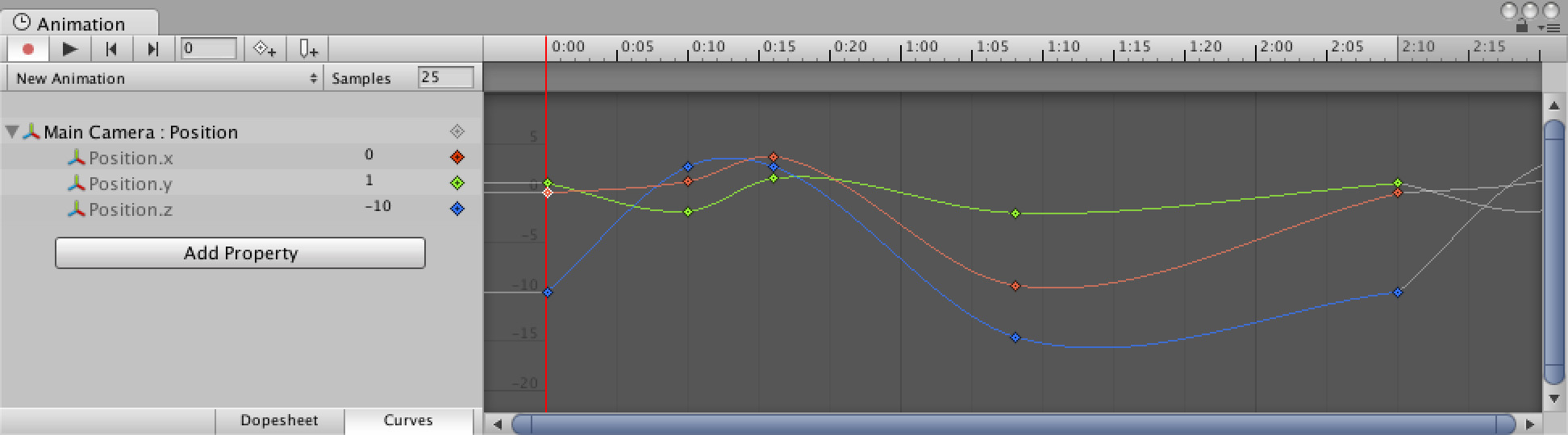
We can easily see that each track has five control points but with a total clip duration of 2.5 seconds (note that the image uses a sample rate of 25 FPS which makes the numbering a bit quirky) we would need 2.5 seconds * 30 frames/second = 75 frames to represent the same data. Even after using linear key reduction, the number of keys would remain higher than five.
As with linear key reduction, our spline control points will have time markers and most of what was mentioned previously will apply to curve fitting as well: we need to search for our neighbour control points, we need to sort our data to be cache efficient, etc.
One important distinction is that while linear key reduction only needed two keys per track to reconstruct our desired value at a particular time T, with curve fitting we might need more. For example, Catmull-Rom splines require four control points. This makes it more likely to increase the amount of cache lines we need to read when we sample our clip. For this reason, and the fact that a spline interpolation function is more expensive to execute, decompression should be slower than with linear key reduction but without access to a solid implementation, the fact that it might be slower is only an educated guess at this point.
Additional Reading
Up next: Signal Processing
Back to table of contents
07 Dec 2016
With simple key quantization, if we needed to sample a certain time T for which we did not have a key (e.g. in between two existing keys), we linearly interpolated between the two.
A natural extension of this is of course to remove keys or key frames which can be entirely linearly interpolated from their neighbour keys as long as we introduce minimal or no visible error.
How It Works
The process to remove keys is fairly straight forward:
- Pick a key
- Calculate the value it would have if we linearly interpolated it from its neighbours
- If the resulting track error is acceptable, remove it
The above algorithm continues until nothing further can be removed. How you pick keys may or may not impact significantly the results. I personally only ever came across implementations that iterated on all keys linearly forward in time. However, in theory you could iterate in any number of ways: random, key with smallest error first, etc. It would be interesting to try various iteration methods.
It is worth pointing out that you need to check the error at a higher level than the individual key you are removing since it might impact other removed keys by changing the neighbour used to remove them. As such you need to look at your error metric and not just the key value delta.
Removing keys is not without side effects: now that our data is no longer uniform, calculating the proper interpolation alpha to reconstruct our value at time T is no longer trivial. To be able to calculate it, we must introduce in our data a time marker per remaining key (or key frame). This marker of course adds overhead to our animation data and while in the general case it is a win, memory wise, it can increase the overall size if the data is very noisy and no or very few keys can be removed.
A simple formula is then used to reconstruct the proper interpolation alpha:
TP = Time of Previous key
TN = Time of Next key
Interpolation Alpha = (Sample Time - TP) / (TN - TP)
Another important side effect in introducing time markers is that when we sample a certain time T, we must now search to find between which two keys we must interpolate. This of course adds some overhead to our decompression speed.
The removal is typically done in one of two ways:
- Removal of whole key frames that can be linearly interpolated
- Removal of independent keys that can be linearly interpolated
While the first is less aggressive and will generally yield a higher memory footprint, the decompression speed will be faster due to needing to search only once to calculate our interpolation alpha.
For example, suppose we have the following track and keys:
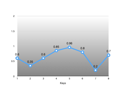
The key #3 is of particular interest:
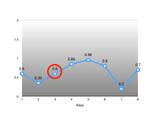
As we can see, we can easily recover the interpolation alpha from its neighbours: alpha = (3 - 2) / (4 - 2) = 0.5. With it, we can perfectly reconstruct the missing key: value = lerp(0.35, 0.85, alpha) = 0.6.
Another interesting key is #4:
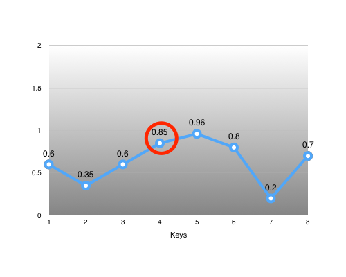
It lies somewhat close to the value we could linearly interpolate from its neighbours: value = lerp(0.6, 0.96, 0.5) = 0.78. Whether the error introduced by removing it is acceptable or not is determined by our error metric function.
In The Wild
This algorithm is perhaps the most common and popular out there. Both Unreal 4 and Unity 5 as well as many popular game engines support this format. They all use slight variations mostly in their error metric function but the principle remains the same. Sadly most implementations out there tend to use a poorly implemented error metric which tends to yield bad results in many instances. This typically stems from using a local error metric where each track type has a single error threshold. Of course the problem with this is that due to the hierarchical nature of our bone data, some bones need higher accuracy (e.g. pelvis, root). Some engines mitigate this by allowing a threshold per track or per bone but this requires some amount of tweaking to get right which is often undesirable and sub-optimal.
Twice in my career I had to implement a new animation compression algorithm and both times were to replace bad linear key reduction implementations.
From the implementations I have seen in the wild, it seems more popular to remove individual keys as opposed to removing whole key frames.
Sadly due to the loss of data uniformity, the cache locality of the data we need suffers. Unlike for simple key quantization, we can no longer simply sort by key frame if we remove individual keys (you still can if you remove whole key frames though) to keep things cache efficient.
Although I have not personally witnessed it, I suspect it should be possible to use a variation of a technique used by curve fitting to sort our data in a cache friendly way. It is well described here and we’ll come back to it when we cover curve fitting.
The need to constantly search for which neighbour keys to use when interpolating quickly adds up since it scales poorly. The longer our clip is, the wider the range we need to search and the more tracks we have also increases the amount of searching that needs to happen. I have seen two ways to mitigate this: partitioning our clip or by using a cursor.
Partitioning our clip data as we discussed with uniform segmenting helps reduce the range to search in as our clip length increases. If the number of keys per block is sufficiently small, searching can be made very efficient with a sorting network or similar strategy. The use of blocks will also decrease the need for precision in our time markers by using a similar form of range reduction which allows us to use fewer bits to store them.
Using a cursor is conceptually very simple. Most clips play linearly and predictably (either forward or backward in time). We can leverage this fact to speed up our search by caching which time we sampled last and which neighbour keys were used to kickstart our search. The cursor overhead is very low if we remove whole key frames but the overhead is a function of the number of animated tracks if we remove individual keys.
Note that it is also quite possible that by using the above sorting trick that it could speed up the search but I cannot speak to the accuracy of this statement at this time.
Even though we can reach a smaller memory footprint with linear key reduction compared to simple key quantization, the amount of cache lines we’ll need to touch when decompressing is most likely going to be higher. Along with the need to search for key neighbours, these facts makes it slower to decompress using this algorithm. It remains popular due to the reduced memory footprint which was very important on older consoles (e.g. PS2 and PS3 era) as well as due to its obvious simplicity.
See the following posts for more details:
Up next: Curve Fitting
Back to table of contents
17 Nov 2016
Once upon a time, sub-sampling was a very common compression technique but it is now mostly relegated to history books (and my boring blog!).
How It Works
It is conceptually very simple:
- Take your source data, either from Maya (3DS Max, etc.) or already sampled data at some sample rate
- Sample (or re-sample) your data at a lower sample rate
Traditionally, character animations have a sample rate of 30 FPS. This means that for any given animated track, we end up with 30 keys per second of animation.
Sub-sampling works because in practice, most animations don’t move all that fast and a lower sampling rate is just fine and thus 15-20 FPS is generally good enough.
Edge Cases
Now of course, this fails miserably if this assumption does not hold true or if a particular key is very important. It can often be the case that an important key is removed with this technique and there is sadly not much that can be done to avoid this issue short of selecting another sampling rate.
It is also worth mentioning that not all sampling rates are necessarily equal. If your source data is already discretized at some original sample rate, sampling rates that will retain whole keys are generally superior to sample rates that will force the generation of new keys by interpolating their neightbours.
For example, if my source animation track is sampled at 30 FPS, I have a key every 1s / 30 = 0.033s. If I sub-sample it at 18 FPS, I have a key every 1s / 18 = 0.055s. This means every key I need is not in sync with my original data and thus new keys must be generated. This will yield some loss of accuracy.
On the other hand, if I sub-sample at 15 FPS, I have a key every 1s / 15 = 0.066s. This means every other key in my original data can be discarded and the remaining keys are identical to my original keys.
Another good example is sub-sampling at 20 FPS which will yield a key every 1s / 20 = 0.05s. This means every 3rd key will be retained from the original data (0.0 … 0.033 … 0.066 … 0.1 … 0.133 … 0.166 … 0.2 …). The other keys do not line up and will be artificially generated from our original neighbour keys.
The problem of keys not lining up is of course absent if your source animation data is not already discretized. If you have access to the Maya (or 3DS Max) curves, the sub-sampling will retain higher accuracy.
In The Wild
In the wild, this used to be a very popular technique on older generation hardware such as the Xbox 360 and the PlayStation 3 (and older). It was very common to keep most of your main character animations with a high sample rate of say 30 FPS, while keeping most of your NPC animations at a lower sample rate of say 15 FPS. Any specific animation that required high accuracy would not be sub-sampled and this selection process was done by hand, making its usage somewhat error prone.
Due to its simplicity, it is also commonly used alongside other compression techniques (e.g. linear key reduction) to further reduce the memory footprint.
However, nowadays this technique is seldom used in large part because we aren’t as constrained by the memory footprint as we used to be and in part because we strive to push the animation quality ever higher.
Up next: Linear Key Reduction
Back to table of contents