15 Nov 2016
Simple quantization is perhaps the simplest compression technique out there. It is used for pretty much everything, not just for character animation compression.
How It Works
It is fundamentally very simple:
- Take some floating point value
- Normalize it within some range
- Scale it to the range of a N bit integer
- Round and convert to a N bit integer
That’s it!
For example, suppose we have some rotation component value within the range [-PI, PI] and we wish to represent it as a signed 16 bit integer:
- Our value is:
0.25
- Our normalized value is thus:
0.25 / PI = 0.08
- Our scaled value is thus:
0.08 * 32767.0 = 2607.51
- We perform arithmetic rounding:
Floor(2607.51 + 0.5) = 2608
Reconstruction is the reverse process and is again very simple:
- Our normalized value becomes:
2608.0 / 32767.0 = 0.08
- Our de-quantized value is:
0.08 * PI = 0.25
If we need to sample a certain time T for which we do not have a key (e.g. in between two existing keys), we typically linearly interpolate between the two. This is just fine because key frames are supposed to be fairly close in time and the interpolation is unlikely to introduce any visible error.
Edge Cases
There is of course some subtlety to consider. For one, proper rounding needs to be considered. Not all rounding modes are equivalent and there are so many!
The safest bet and a good default for compression purposes, is to use symmetrical arithmetic rounding. This is particularly important when quantizing to a signed integer value but if you only use unsigned integers, asymmetrical arithmetic rounding is just fine.
Another subtlety is whether to use signed integers or unsigned integers. In practice, due to the way two’s complement works and the need for us to represent the 0 value accurately, when using signed integers, the positive half and the negative half do not have the same size. For example, with 16 bits, the negative half ranges from [-32768, 0] while the positive half ranges from [0, 32767]. This asymmetry is generally undesirable and as such using unsigned integers is often favoured. The conversion is fairly simple and only requires doubling our range (2 * PI in the example above) and offsetting it by the signed ranged (PI in the example above).
- Our normalized value is thus:
(0.25 + PI) / (2.0 * PI) = 0.54
- Our scaled value is thus:
0.54 * 65535.0 = 35375.05
- With arithmetic rounding:
Floor(35375.05 + 0.5) = 35375
Another point to consider is: what is the maximum number of bits we can use with this implementation? A single precision floating point value can only accurately represent up to 6-9 significant digits as such the upper bound appears to be around 19 bits for an unsigned integer. Higher than this and the quantization method will need to change to an exponential scale, similar to how depth buffers are often encoded in RGB textures. Further research is needed on the nuances of both approaches.
In The Wild
The main question remaining is how many bits to use for our integers. Most standalone implementations in the wild use the simple quantization to replace a purely raw floating point format. Tracks will often be encoded on a hardcoded number of bits, typically 16 which is generally enough for rotation tracks as well as range reduced translation and scale tracks.
Most implementations that don’t exclusively rely on simple quantization but use it for extra memory gains again typically use a hardcoded number of bits. Here again 16 bits is a popular choice but sometimes as low as 12 bits is used. This is common for linear key reduction and curve fitting. Wavelet based implementations will typically use anywhere between 8 and 16 bits per coefficient quantized and these will vary per sub-band as we will see when we cover this topic.
The resulting memory footprint and the error introduced are both a function of the number of bits used by the integer representation.
This technique is also very commonly used alongside other compression techniques. For example, the remaining keys after linear key reduction will generally be quantized as will curve control points after curve fitting.
This algorithm is very fast to decompress. Only two key frames need to be decompressed and interpolated. Each individual track is trivially decompressed and interpolated. It is also terribly easy to make the data very processor cache friendly: all we need to do is sort our data by key frame, followed by sorting it by track. With such a layout, all our data for a single key frame will be contiguous and densely packed and the next key frame we will interpolate will follow as well contiguously in memory. This makes it very easy for prefetching to happen either within the hardware or manually in software.
For example, suppose we have 50 animated tracks (a reasonable number for a normal AAA character), each with 3 components, stored on 16 bits (2 bytes) per component. We end up with 50 * 3 * 2 = 300 bytes for a single key frame. This yields a small number of cache lines on a modern processor: ceil(300 / 64) = 5. Twice that amount needs to be read to sample our clip.
Due in large part to the cache friendly nature of this algorithm, it is quite possibly the fastest to decompress.
My GDC presentation goes in further depth on this topic, its content will find its way here in due time.
Up next: Advanced Quantization
Back to table of contents
13 Nov 2016
Over the years, a number of techniques have emerged to address the problem of character animation compression. These can be roughly broken down into a handful of general families:
Note that simple quantization and sub-sampling can be and often are used in tandem with the other three compression families although they can be used entirely on their own.
Up next: Simple Quantization
Back to table of contents
10 Nov 2016
Uniform segmenting is performed by splitting a clip into a number of blocks of equal or approximately equal size. This is done for a number of reasons.
Range Reduction
Splitting large clips (such as cinematics) into smaller blocks allows us to use range reduction on each track within a block. This can often help reach higher levels of compression especially on longer clips. This is typically done on top of the clip range reduction to further increase our compression accuracy.
Easier Seeking
For some compression algorithms, seeking is slow because it involves searching for the keys or control points surrounding the particular time T we are trying to sample. Techniques exist to speed this up by using optimal sorting but it adds complexity. With blocks sufficiently small (e.g. 16 key frames), optimal sorting might not be required nor the usage of a cursor (cursors are used by these algorithms to keep track of the last sampling performed to accelerate the search of the next sampling). See the posts about linear key reduction and curve fitting for details.
With uniform segmenting, finding which blocks we need is very fast in large part because there are typically few blocks for most clips.
Streaming and TLB Friendly
The easier seeking also means the clips are much easier to stream. Everything you need to sample a number of key frames is bundled together into a single contiguous block. This makes it easy to cache them or prefetch them during playback.
For similar reasons, this makes our clip data more TLB friendly. All our relevant data needed for a number of key frames will use the same contiguous memory pages.
Required For Wavelets
Wavelet functions typically work on data whose’s size is a power of two. Some form of padding is used to reach a power of two when the size doesn’t match. To avoid excessive padding, clips are split into uniform blocks. See the post about wavelet compression for details.
Downsides
Segmenting a clip into blocks does add some amount of memory overhead:
- Each clip will now need to store a mapping of which block is where in memory.
- If range reduction is done per block as well, each block now includes range information.
- Blocks might need a header with some flags or other relevant information.
- And for some compression algorithms such as curve fitting, it might force us to insert extra control points or to retain more key frames.
However, the upsides are almost aways worth the hassle and overhead.
Up next: Main Compression Families
Back to table of contents
09 Nov 2016
Range reduction is all about exploiting the fact that the values we compress typically have a much smaller range in practice than in theory.
For example, in theory our translation track range is infinite but in practice, for any given clip, the range is fixed and generally small. This generalizes to rotation and scale tracks as well.
How It Works
First we start with some animated translation track.
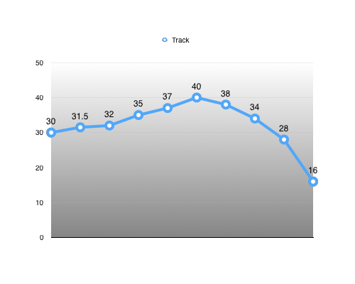
Using this track as an example, we first find the minimum and maximum value that will bound our range: [16, 40]
Using these, we can calculate the range extent: 40 - 16 = 24
Now, we have everything we need to re-normalize our track. For every key: normalized value = (input value - range minimum) / range extent
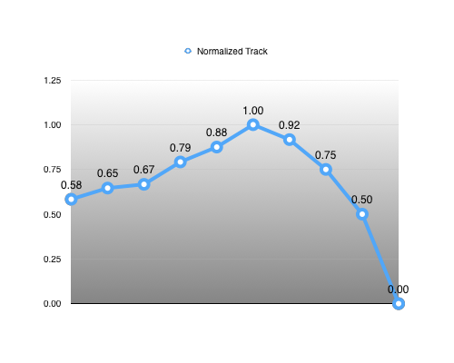
Reconstructing our input value becomes trivial: input value = (normalized value * range extent) + range minimum
We thus represent our range as a tuple: (range minimum, range extent) = (16, 24)
This representation has the advantage that reconstructing our input value is very efficient and can use a single fused multiply-add instruction when it is available (and it is on modern CPUs that support FMA as well as modern GPUs).
This increases the information we need to keep around by an extra tuple for every track. For example, a translation track would require a pair of Vector3 values (6 floats) to encode our 3D range.
This extra information allows us to increase our accuracy (sometimes dramatically). While both representations are 100% equivalent mathematically, this only holds true if we have infinite precision. In practice, single precision floating point values only have 6 to 9 significant decimal digits of precision. Typically, our original input range will be much larger than our normalized range and as such its precision will be lower.
This is most easily visible when our track needs to be quantized on a fixed number of bits. For example, our example translation track would typically be bounded by a large hardcoded number such as 100 centimetres. Our hardcoded theoretical track range thus becomes: [-100, 100]. Tracks with values outside of this range can’t be represented and might need a different base range or a raw un-quantized format. The above range is thus represented by the tuple: (-100, 200). If we quantized this range on 16 bits, our input range of 200cm is evenly divided by 65536 which gives us a precision of: 200cm / 65536 = 0.003cm. However, because we know the range is much smaller, using the same number of bits yields a precision of: 1.0 / 65536 = 0.000015 * 24cm = 0.00037cm. Our accuracy has increased by 8x!
In practice, rotation tracks are generally bounded by [-PI, PI] but animated bones will only use a very small portion of that range on any given clip. Similarly, translation tracks are typically bounded by some hardcoded range but only a small portion is ever used by most bones. This translates naturally to scale tracks as well.
A side effect of range reduction is that all tracks end up being normalized. This is important for the simple quantization compression algorithms as well as when wavelets are used on an aggregate of tracks (as opposed to per track). Future posts will go further into detail.
Conclusion
Range reduction allows us to focus our precision on the range of values that actually matters to us. This increased accuracy very often allows us to be more aggressive in our compression, reducing our overall size despite any extra overhead.
Do note that the extra range information does add up and for very short clips (e.g. 4 key frames) this extra overhead might yield a higher overall memory footprint. These are typically uncommon enough that it is simpler to accept that occasional loss in exchange for simpler decompression that can assume that all tracks use range reduction.
Up next: Uniform Segmenting
Back to table of contents
03 Nov 2016
One of the primary advantage of storing bone transforms in local space as opposed to object space is that it reduces dramatically the amount of data that changes. For example, if we have two bones connected, and they have their local rotation animated, we end up with two animated tracks in local space, but three tracks in object space. This is true because the rotation changes from the root bone will cause a translation offset on the second bone.
It is also the case that many bones are never animated by a majority of clips. For example, inverse kinematic (IK) bones are only ever animated when they are required (e.g. object pick up) and facial bones are typically used by cinematic clips or overlay clips. When bones aren’t animated, they will be by definition constant in our raw data.
Consequently, it is often the case that tracks are constant. In general, character animations end up animating many more rotation tracks than they do for translation or scale. As such, translation and scale tracks often end up entirely constant in a clip. Taking advantage of this can be done in one of two ways:
- Implicitly: linear key reduction will typically reduce such tracks to two keys since everything else can be interpolated (curve fitting and wavelet benefit similarly from this)
- Explicitly: by using a bit set that marks tracks as constant or variable
Typically, using a bit set and explicitly dropping constant tracks is the superior method to reduce the memory footprint but it does add a bit more complexity to the decompression algorithm. It is entirely worth it in my opinion.
Constant tracks will come in two forms:
- Constant and equal to the default track value (typically equal to the bind pose or identity)
- Constant and equal to some arbitrary track value
For obvious reasons, these tracks compress very well. In the first case, we only need to store a single bit per track. If a track is constant, we easily know which value it should have based on the track type (rotation, translation, or scale). In the second case, in addition to our single bit per track, we also need to store our single repeated key value. This single key can be stored raw since its memory footprint overall will remain small regardless or you can quantize it on fewer bits.
My GDC presentation will include real numbers on the frequency of constant bones, constant tracks, and constant track components from a modern untitled AAA video game but I cannot include them here just yet.
In my experience, the number of constant tracks is closely correlated by the number of constant track components (e.g. a constant scale track is equivalent to three constant scale track components). As such any extra gains we might have from using a bit set per track component (instead of per track) is likely to be offset by the larger bit set size and the extra complexity will likely make decompression slower.
See also Animation Data in Numbers
Up next: Range Reduction
Back to table of contents