30 Aug 2017
While investigating precision issues with ACL, I ran into two problems that I hadn’t seen documented elsewhere and that slightly surprised me.
Dot product
Calculating the dot product between two vectors is a very common operation used for all sorts of things. In an animation compression library, it’s primary use is normalizing quaternions. Due to the nature of the code, accuracy is very important as it can impact the final compressed size as well as the resulting decompression error.
SSE 4 introduced a dot product instruction: DPPS. It allows the generated code to be more concise and compact by using fewer registers and instructions. I won’t speak to its performance here but sadly; its accuracy is not good enough for us by a tiny, yet important, sliver.
For the purpose of this blog post, we will use the following nearly normalized quaternion as an example: { X, Y, Z, W } = { -0.6767403483, 0.7361232042, 0.0120376134, -0.0006215832 }. This is a real quaternion from a real clip of the Carnegie-Mellon University (CMU) motion capture database that proved to be problematic. With doubles, the dot product is 1.0000001612809224.
Using plain C++ yields the following code and assembly (compiled with AVX support under Visual Studio 2015 with an x64 target):
- The result is: 1.00000024. Not quite the same but close.
Using the SSE 4 dot product instruction yields the following code and assembly:
- The result is: 1.00000024.
Using a pure SSE 2 implementation yields the following assembly:
- The result is: 1.00000012.
These are all nice but it isn’t immediately obvious how big the impact can be. Let’s see how they perform after taking the square root (note that the SSE 2 SQRT instruction is used here):
- C++: 1.00000012
- SSE 4: 1.00000012
- SSE 2: 1.00000000
Again, these are all pretty much the same. What happens when we take the square root reciprocal after 2 iterations of Newton-Raphson?
- C++: 0.999999881
- SSE 4: 0.999999881
- SSE 2: 0.999999940
With this square root reciprocal, here is how our quaternions look after being multiplied to normalize them and their associated dot product.
- C++:
{ -0.676740289, 0.736123145, 0.0120376116, -0.000621583138 } = 0.999999940
- SSE 4:
{ -0.676740289, 0.736123145, 0.0120376116, -0.000621583138 } = 1.00000000
- SSE 2:
{ -0.676740289, 0.736123145, 0.0120376125, -0.000621583138 } = 0.999999940
Here is the dot product calculated with doubles:
- C++: 0.99999999381912441
- SSE 4: 0.99999999381912441
- SSE 2: 0.99999999384079208
And the new square root:
- C++: 0.999999940
- SSE 4: 1.00000000
- SSE 2: 0.999999940
Now the new reciprocal square root:
- C++: 1.00000000
- SSE 4: 1.00000000
- SSE 2: 1.00000000
After all of this, our delta from a true length of 1.0 before (as calculated with doubles) was 1.612809224e-7 before normalization. Here is how they fare afterwards:
- C++: 6.18087559e-9
- SSE 4: 6.18087559e-9
- SSE 2: 6.15920792e-9
And thus, the difference between using SSE 4 and SSE 2 is just 2.166767e-11.
As it turns out, the SSE 2 implementation appears the most accurate one and yields the lowest decompression error as well as a smaller memory footprint (by a tiny bit).
Normalizing a quaternion
There are two mathematically equivalent ways to normalize a quaternion: taking the dot product, calculating the square root, and dividing the quaternion with the result, or taking the dot product, calculating the reciprocal square root, and multiplying the quaternion with the result.
Are the two methods equivalent with floating point mathematics? Again, we will not discuss the performance implications as we are only concerned with accuracy here. Using the previous example quaternion and using the SSE 2 dot product yields the following result with the first method:
- Dot product: 1.00000012
- Length:
sqrt(1.00000012) = 1.00000000
- Normalized quaternion using division:
{ -0.6767403483, 0.7361232042, 0.0120376134, -0.0006215832 }
- New dot product: 1.00000012
- New length: 1.00000000
And now using the reciprocal square root with 2 Newton-Raphson iterations:
- Dot product: 1.00000012
- Reciprocal square root: 0.999999940
- Normalized quaternion using multiplication:
{ -0.676740289, 0.736123145, 0.0120376125, -0.000621583138 }
- New dot product: 0.999999940
- New length: 0.999999940
- New reciprocal square root: 1.00000000
By using the division, normalization fails to yield us a more accurate quaternion because of square root is 1.0. The reciprocal square root instead allows us to get a more accurate quaternion as demonstrated in the previous section.
Conclusion
It is hard to see if the numerical difference is meaningful but over the entire CMU database, both tricks together help reduce the memory footprint by 200 KB and lower our error by a tiny bit.
For most game purposes, the accuracy implication of these methods does not matter all that much and rarely have a measurable impact. Picking whichever method is fastest to execute might just be good enough.
But when accuracy is of a particular concern, special care must be taken to ensure every bit of precision is retained. This is one of the motivating reasons for ACL having its own internal math library: granular control over performance and accuracy.
13 Apr 2017
In modern video games, the 4x4 matrix multiplication is an important cornerstone. It is used for a very long list of things: moving individual character joints, physics simulation, rendering, etc. To generate a single video game image (and we typically generate between 25 and 60 per second), several thousand matrix multiplications will take place. Today, we will take an in-depth look at such a fundamental piece of code.
As I will show, we can improve on some of the most common implementations out in the wild. I will use DirectX Math as a reference here but I have seen identical implementations in many state of the art game engines.
This blog post will be broken down into four sections:
Note that all the code for this can be found here. Feel free to toy with it and replicate the results or contribute your own.
Our test cases
In order to keep our observations grounded in reality, we will use three test cases that represent common heavy usage of 4x4 matrix multiplication. These are very synthetic in nature but they will make profiling and measuring immensely easier. Modern game engines do many things with many threads which can make profiling on PC somewhat a bit more complicated especially for something as short and simple as matrix multiplication.
Test case #1
Our first test case applies a constant matrix to an array of 64 matrices. Aside from our constant matrix, each input will be read from memory (here everything fits in our processor cache but it doesn’t matter much) and each output will be written back to memory. This code is meant to simulate the common operation of transforming an array of object space matrices into world space matrices, perhaps for skinning purposes.
Test case #2
Our second test case transforms an array of 64 local space matrices into an array of 64 object space matrices. To perform this operation, each local space matrix is multiplied by the parent object space matrix. The root matrix is trivial and equal in both local and object space as it has no parent. In this contrived example the parent matrix is always the previous entry in the array but in practice it would be some arbitrary index previously transformed. This operation is common at the end of the animation runtime where the pose generated will typically be in local space.
Test case #3
Our third test case takes two constant matrices and writes the result to a static array. The array is made static to prevent the compiler from stripping the code. This code is synthetic and meant to try and profile one off multiplications that happen everywhere in gameplay code. We perform the operation 64 times to help us measure the impact since the code is very fast to begin with.
Function signature variations
Our reference implementation taken from DirectX Math has the following signature:
There a few things that are noteworthy here. The function is marked inline but due to its considerable size, the function is generally never inlined. It also uses the __vectorcall calling convention with the macro XM_CALLCONV. This allows up to 6 SIMD input arguments to be passed by register (the default calling convention passes them by value on the stack, unlike with PowerPC) and the return value can also be up to 4 SIMD outputs passed by register. This also works for aggregate types such as XMMatrix. The function takes 2 arguments: M1 is passed by register with the help of FXMMATRIX and M2 is passed by const & with the help of CXMMATRIX.
This function signature will be called in our data: reg
We can vary the function signature in a number of ways and it will be interesting to compare the results. I came up with a number of variations. They are as follow.
Force inline
As mentioned, since our function is very large, inlining will typically fail to happen. However in very hot code, it still makes sense to inline the function.
This function signature will be called: inl
Pass everything from memory
An obvious change we can make is to pass both input arguments as const &. In many cases our matrices might not be cached in local registers to begin with and we have to load them from memory anyway (such as in test case #2).
This function signature will be called: mem
Flip our matrix arguments
In our matrix implementation, the rows of M2 are multiplied whole with each matrix element from M1. The code ends up looking like this:
This repeats 4 times for each row of M1. It is obvious that we can cache our 4 values from M2 and indeed the compiler typically does so for us in our reference implementation. Each of those 4 rows will be needed again and again but the same cannot be said of the 4 rows of M1 which are only needed temporarily. It would thus make sense to pass the matrix arguments in the opposite order: M2 first by register and M1 second by const &.
Note that we use a macro to perform the flip cleanly. I would have preferred a force inlined function but the compiler was not generating clean assembly from it.
This function signature will be called: flip
Expanded matrix argument
Even though the __vectorcall calling convention conveniently passes our matrix in 4 registers, it might help the compiler make different decisions if we are explicit about our intentions.
Our expanded variant will always use the flipped argument ordering. Measuring the non-flipped ordering is left as an exercise to the reader.
This function signature will be called: exp
Return value by argument
Another thing that is very common for a matrix multiplication implementation is to have the return value as a pointer or reference in a third argument.
Again this might help the compiler make different optimization choices. Note as well that implementations with this variant must explicitly cache the rows of M2 in order to have the correct result in case where the result is written to M2. It also improves the generated assembly as otherwise the output matrix would alias the arguments causing the compiler to not perform the caching automatically for you.
This function signature can be applied to all our variants and it will add the suffix 2
Permute all the things!
Taking all of this together and permuting everything yields 12 variants as follow:
In our data, they are called:
- reg
- reg2
- reg_flip
- reg_flip2
- reg_exp
- reg_exp2
- mem
- mem2
- inl
- inl2
- inlexp
- inlexp2
Hopefully this covers a large extent of common and sensible variations.
Our competing implementations
I was able to come up with six distinct implementations of the matrix multiplication, including the original reference. Note that I did not attempt to make the fastest implementation possible, there are other things we could try to make them faster. I also made sure that each version gave a result that was a exactly the same as the reference implementation, down to the last bit (binary exact).
Reference
The reference implementation is quite large as such I will not include the full source here but the code can be found here.
The reference regexp2 variant uses 10 XMM registers and totals 70 instructions.
Broadcast
In our reference implementation, an important part can be tweaked a bit.
We load a row from M1, extract each component, and replicate it into the 4 lanes of our SIMD register. This will compile down to 1 load instruction followed by 4 shuffle instructions. This was very common on older consoles: loads from memory were very expensive and none of the other instructions could work directly from memory. However, on SSE and in particular with AVX, we can do a bit better. We can use the _mm_broadcast_ss instruction. It takes as input a pointer to a scalar floating point value and it will output the replicated value over our 4 SIMD lanes. We thus save and avoid our load instruction.
The code for this variant can be found here.
The version 0 regexp2 variant uses 7 XMM registers and totals 58 instructions.
Looping
Another change we can perform is inspired from this post on StackOverflow. I rewrote the assembly into C++ code that uses intrinsics to try and keep it comparable.
Two versions were written: version 2 uses load/shuffle (code here) and version 1 uses broadcast (code here).
Branching was notoriously slow on the old consoles, it will be interesting to see how newer hardware performs.
The version 1 regexp2 variant uses 7 XMM registers and totals 23 instructions.
The version 2 regexp2 variant uses 10 XMM registers and totals 37 instructions.
Handwritten assembly
Similar to our looping versions, I also kept the hand written assembly version referenced. I made a few tweaks to make sure the results were binary exact. Sadly, the tweaks required the usage of one extra register. Having run out of volatile registers, I elected to load the first row of M2 directly from memory with the multiply instruction during every iteration.
Only two variants were implemented: regexp2 and mem2.
Two versions were written: version 3 uses load/shuffle (code here) and version 4 uses broadcast (code here).
The version 3 regexp2 variant uses 5 XMM registers and totals 21 instructions.
The version 4 regexp2 variant uses 5 XMM registers and totals 17 instructions.
The results
For our purposes, each test will be run 1000000 times and the cumulative time will be considered to be 1 sample. We will repeat this to gather 100 samples. To avoid skewing in our data that might result from various external sources (CPU frequency changes, other OS work, etc.), we will retain and use the 80th percentile from our dataset. Due to the simple nature of the code, this should be good enough for us to draw meaningful conclusions. All measurements are in milliseconds.
All of my raw results are parsed with a simple python script to extract the desired percentile and format it in a table form. The script can be found here.
I ran everything on my desktop computer which has an Intel i7-6850K processor. While my CPU differs from what the Xbox One and PlayStation 4 use, they both support AVX and could benefit from the same changes.
I also measured running the test cases with multithreading enabled to see if the results were consistent. Since the results were indeed consistent, we will only talk about the single threaded case but all the data for the test results can be found here:
Test case results
Here are the results for our 3 test cases:
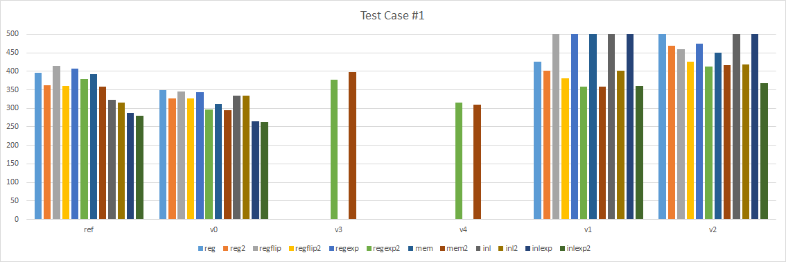
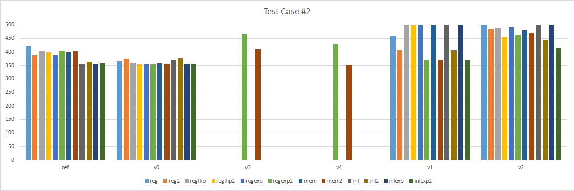
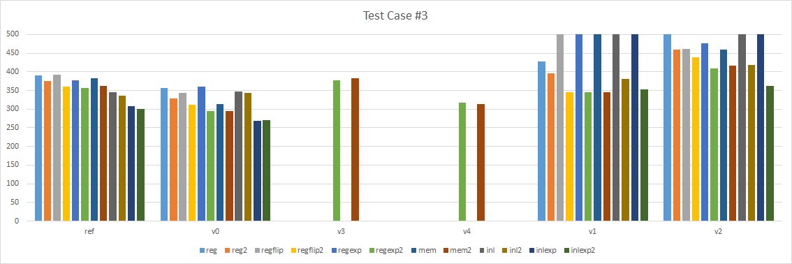
A few things are immediately obvious:
- Version 1 and 2, the looping intrinsic versions, are terribly slow. I moved them to the right so we can focus on the left part.
- Version 0 is consistently faster than our reference implementation.
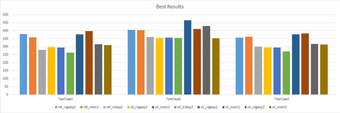
Here are the same results but only considering the best 3 variants (regexp2, mem2, and inlexp2) and the best 4 versions (reference, version 0, version 3, and version 4).
Load/shuffle versus broadcast
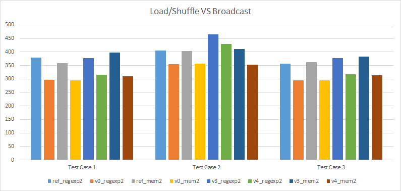
Overwhelmingly, we can see that the versions that use broadcast are faster than their counterpart that uses load/shuffle. This is not too surprising: we use fewer registers, as a result fewer registers spill on the stack, and fewer instructions are used. This is more significant when the function isn’t force inlined since in our test cases, whatever we spill on the stack ends up hoisted outside of our loops when inlined.
The fact that we use fewer registers and instructions also has other side effects, namely it can help the compiler to inline functions. In particular, this is the case for version 1 and 2: version 1 uses broadcast and gets inlined automatically while version 2 uses load/shuffle and does not get inlined.
Output in registers versus memory
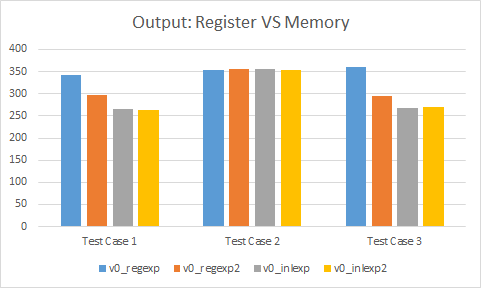
For test cases #1 and #3, passing our return value as an argument is a net win when there is no inlining. This remains true to a lesser extent even when the functions are force inlined which means it helps the compiler make better choices.
However, for test case #2, it can sometimes be a bit slower. It seems that the assembly generated at the call site isn’t as clean as it could be. It’s possible that by tweaking the test case code a bit, performance could be improved.
Flipped versus expanded
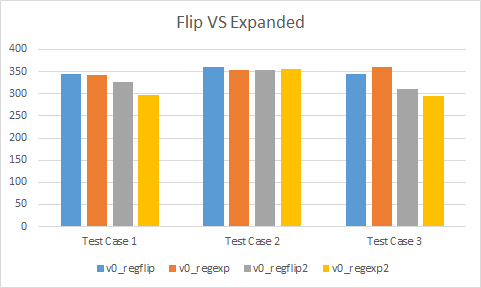
Looking only at version 0, the behaviour seems to differ depending when the result is passed as an argument or by register. In the regflip and regexp variants, performance can be faster (test case #2), the same (test case #1), or slower (test case #3). It seems there is high variability with what the compiler chooses to do. On the other hand, with the regflip2 and regexp2 variants, performance is generally faster. Test case #2 has about equal performance but as we have seen, that test case seems to favour results being returned by register.
Inlining
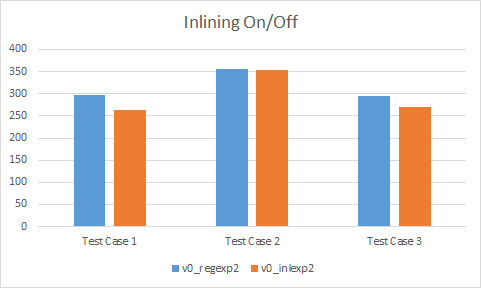
As it turns out, inlining sometimes gives a massive performance gain and sometimes it comes down to about the same. In general, it is best to let the compiler make inlining decisions but sometimes in very hot code, it is desirable to manually force the inlining for performance reasons. It thus makes sense to provide at least 2 versions of matrix multiplication: with and without force inlining.
Looping
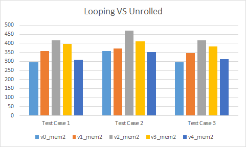
The looping versions are quite interesting. The 2 versions that use intrinsics perform absolutely terribly. They are worse by far, generally breaking out of the charts above. Strangely, they seem to benefit massively from passing the result as an argument (not shown on the graph above). Even with the handwritten assembly versions, we can see that they are generally slower than our unrolled intrinsic version 0. As it turns out, branching is still not a great idea in hot code even with modern hardware.
Is handwritten assembly worth it?
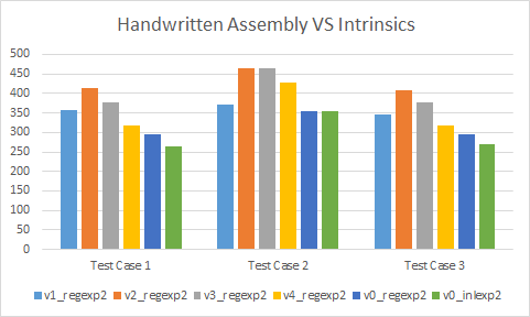
Looking at our looping versions, it is obvious that carefully crafting the assembly by hand can still give significant results. However, we must be careful when doing so. In particular, with Visual Studio, hand written assembly functions will never be inlined in x64, even by the linker. Something to keep in mind.
Best of the best
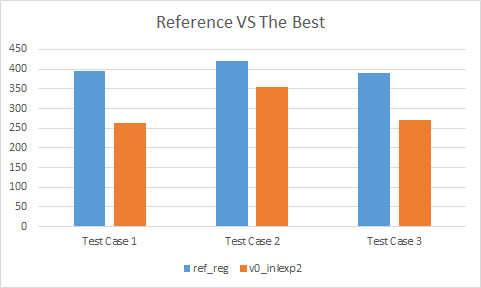
In our results, a clear winner stands above all others: version 0 inlexp2:
- In test case #1, it is 34% faster then the reference implementation
- In test case #2, it is 16% faster then the reference implementation
- In test case #3, it is 31% faster then the reference implementation
Even when it isn’t the fastest implementation, it is within measuring error of the leading alternative. And that leading alternative is always a variant of version 0.
Conclusion
As demonstrated by our data, even a hyper optimized piece of code such as matrix multiplication can sometimes be improved by new hardware features such as the AVX broadcast instruction. In particular, the broadcast instruction allows us to reduce register pressure which avoids spilling registers on the stack and saves on the corresponding instructions that do so. On a platform such as x64, register pressure is a real and important problem that must be taken into account for complex and hot code.
From our results, it seems to make sense to provide 2 implementations for matrix multiplication:
- One of regflip2, regexp2, or mem2 that does not force inlining, suitable for everyday usage
- inlexp2 that forces inlining, perfect for that piece of hot code that needs to save every cycle
This keeps things simple for the user: all variants return the result in a 3rd argument. Macros can be used to keep things clean and fast.
As always with optimizations, it is important to measure often and to never blindly make a change without measuring first.
DirectX Math commit d1aa003
11 Apr 2017
For a very long time now with every new gaming console generation came a new set of hardware. New hardware meant new constraints which meant we had to revisit old optimization tricks, rules, and popular beliefs.
With the latest generation, both leading consoles (Xbox One and PlayStation 4) have opted for x64 and AMD CPUs. These are indeed significantly different from the old PowerPC CPUs used by Xbox 360 and PlayStation 3.
I spent a significant amount of time last year optimizing cloth simulation code that had been written in mind for the previous generation and with a few tweaks I was able to get decent gains on the latest hardware. Unfortunately that code was proprietary and as such I cannot use it to show the changes and lessons I learned. Instead, I will take the decent and well respected DirectX Math public library and highlight as well as optimize specific examples.
Due to the large amount of code, charts, and information required to properly explain everything, this topic will be split into several parts:
Hardware highlights
The PowerPC era
In the Xbox 360 and PlayStation 3 generation, both CPUs were quite different, in particular the PlayStation 3 CPU was a significant departure from modern trends at the time. We will focus on it today only because it has been more publicly documented than its counterpart and the lessons we’ll learn from it applied to both consoles.
The PlayStation 3 console sported a fancy Cell microprocessor. We will not focus on the multi-threading aspects in this post series and instead take a deeper look at the execution of a single thread at the assembly level. One important characteristic of PowerPC chips is that they are based on the RISC model. RISC hardware is generally known to have more user addressable registers than CISC, the variant used by Intel and AMD for modern x64 CPUs. In fact, PowerPC CPUs have 32 general purpose registers, 32 floating point registers, and 32 AltiVec SIMD registers (note that the Cell SPEs had 128 registers!). Both consoles also had cache lines that were 128 bytes wide and their CPUs did not support out-of-order execution.
This gave rise to two common techniques to optimize code at the assembly level that we will revisit in this series.
First, the large amount of registers meant that we could leverage them easily to mitigate the fact that loading values from memory was slow and could not be easily hidden due to the in-order nature of the execution. This lead to register packing: a technique where values are loaded first in bulk as part of a vector value and specific components are extracted on demand.
Second, because the register sets for floating point and SIMD math were different, moving a value from one set to another involved storing the value in memory (generally the stack) and reloading it. This led to what is commonly known as load-hit-store stalls. To mitigate this, whenever SIMD math was mixed with scalar math it was generally best to treat simple scalar floating point math as if it were SIMD: the same scalar was replicated to every SIMD lane.
It is also worth noting that the calling convention used on those consoles favours passing many arguments by register, including vector arguments. There are also many other peculiarities that affected how code should best be written for the hardware such as avoiding to stress the poor branch prediction but we will not cover these at this time.
The x64 SSE era
The modern Xbox One and PlayStation 4 consoles opted for x64 AMD CPUs. These are state of the art processors with out-of-order execution, powerful branch prediction, and a large set of instructions from SSE and AVX. These CPUs depart from the previous generation significantly in the number of registers they have: 16 general purpose registers and 16 SIMD registers. The cache lines are also standard in size: 64 bytes wide.
The greatly reduced number of registers means that x64 code is much more prone to register pressure issues. Whenever the number of registers needed goes above 16, registers will spill on the stack, degrading performance. In practice, it isn’t a huge issue in large part because x64 supports instructions that directly work from memory, avoiding the need for a separate load instructions (unlike PowerPC CPUs). For example, in the expression C = add(A, B), A and B can both be residing in registers or B could optionally be a memory address. Internally the CPU has much more than 16 registers and thanks to register renaming and compound CISC instructions, our add instruction will end up performing a load for us behind the scenes. Leveraging this can be very important in hot code as we will see in this series.
Another important characteristic of x64 is that scalar floating point math uses the SSE registers. This means that unlike with PowerPC, converting a floating point value into a SIMD value is very cheap (it could be free if you hand write assembly but compilers will generally generate a shuffle instruction regardless of whether or not you need all components). On the other hand, converting a SIMD value into a floating point value is entirely free and no instruction is generated by modern compilers. This is an important factor to take into account and as we will see later in this series, it can be leveraged to great effect.
Up next
In the next post we will take a deep look at how 4x4 matrix multiplication is performed in DirectX Math and how we can speed it up in various ways.