Animation Compression: Signal Processing
19 Dec 2016Signal processing algorithm variants come in many forms but the most common and popular approach is to use Wavelets. Having utilized this method for all character animation clips on all supported platforms for Thief (2014) I have a fair amount to share with you.
Other signal processing algorithm variants include Discrete Cosine Transform, Principal Component Analysis, and Principal Geodesic Analysis.
The latter two variants are commonly used alongside clustering and database approaches which I’ll explore if enough interest is expressed but I’ll be focusing on Wavelets here.
How It Works
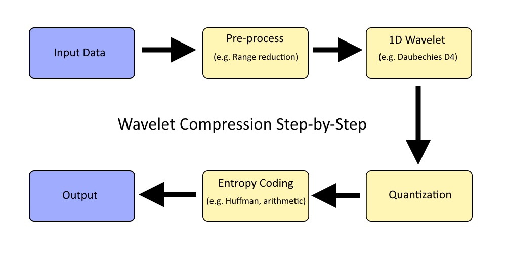
At their core implementations that leverage wavelets for compression will be split into four distinct steps:
- Pre-processing
- The wavelet transform
- Quantization
- Entropy coding
The flow of information can be illustrated like this:
The most important step is, of course, the wavelet function, around which everything is centered. Covering the wavelet function first will help clarify the purpose of every other step.
Aside from quantization all of the steps involved are effectively lossless and only suffer from minor floating point rounding. By altering how many bits we use for the quantization step we can control how aggressive we want to be with compression.
The decompression is simply the same process of steps performed in reverse order.
Wavelet Basics
We will avoid going too in depth on this topic in this series instead we will focus on discussing the wavelet properties and what they mean for us with respect to character animation and compression in general. A good starting point for the curious would be the Haar wavelet which is the simplest of wavelet functions, however, it’s generally avoided for compression.
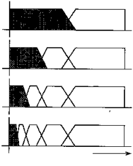
By definition wavelet functions are recursive. Each application of the function is referred to as a sub-band and will output an equal number of scale and coefficient values each exactly half the original input size. In turn, we can recursively apply the function on the resulting scale values of the previous sub-band. The end result is a single scale value and N - 1 coefficients where N is the input size.
Haar wavelet scale is simply the sum of two input values and the coefficient represents their difference. As far as I know most wavelet functions function similarly which yield coefficients that are as close to zero as possible and exactly zero for a constant input signal.
The reason the Haar wavelet is not suitable for compression because it has a single vanishing moment. This means input data is processed in pairs, each outputting a single scale and a single coefficient. The pairs never overlap which means that if there is a discontinuity in between two pairs it will not be taken into account and yield undesirable artifacts if the coefficients are not accurate. A decent alternative is to use a Daubechies D4 wavelet. This is the function I used on Thief (2014) and it turned out quite decently for our purposes.
The wavelet transform can be entirely lossless by using an integer variant but in practice, an ordinary floating point variant is appropriate since compression is lossy by nature and the rounding will not measurably impact the results.
Since wavelet function decomposes a signal on an orthonormal basis we will be able to achieve the highest compression by considering as much of the signal as possible not unlike principal component analysis. Simply concatenate all tracks together into a single 1D signal. The upside of this is that by considering all data as a whole we can find a single orthonormal basis which will allow us to quantize more aggressively but by having a larger signal to transform the decompression speed will suffer. To keep the process reasonably fast in practice on modern hardware each track would likely be processed independently in a small power of two, such as 16 keys at a time. For Thief (2014), all rotation tracks and translation tracks were aggregated independently up to a maximum segment size of 64 KB. We ran the wavelet transform once for rotation tracks, and once for translation tracks.
Pre-processing
Because wavelet functions are recursive the size of the input data needs to be a power of two. If our size doesn’t match we will need to introduce some form of padding:
- Pad with zeroes
- Repeat the last value
- Mirror the signal
- Loop the signal
- Something even more creative?
Which padding approach you choose is likely to have a fairly minimal impact on compression. Your guess is as good as mine regarding which is best. In practice, it’s best to avoid padding as much as possible by keeping input sizes fairly small and processing the input data in blocks or segments.
The scale of output coefficients is a function of the scale and smoothness of our input values. As such it makes sense to perform range reduction and to normalize our input values.
Quantization
After applying the wavelet transform the number of output values will match the number of input values. No compression has happened yet.
As mentioned previously our output values will be partitioned into sub-bands, and a single scale value somewhat centered around zero — both positive and negative. Each sub-band will end up with a different range of values. Larger sub-bands resulting from the first applications of the wavelet function will be filled with high-frequency information while the smaller sub-bands will comprise the low-frequency information. This is important. It means that a single low-frequency coefficient will impact a larger range of values after performing the inverse wavelet transform. Because of this low-frequency coefficients need higher accuracy than high-frequency coefficients.
To achieve compression we will quantize our coefficients into a reduced number of bits while keeping the single scale value with full precision. Due to the nature of the data, we will perform range reduction per sub-band and normalize our values between [-1.0, 1.0]. We only need to keep the range extent for reconstruction and simply assume that the range is centered around zero. Quantization might not make sense for the lower frequency sub-bands with 1, 2, 4 coefficients due to the extra overhead of the range extent. Once our values are normalized we can quantize them. To choose how many bits to use per coefficient we can simply hard code a high number such as 16 bits, 12 bits, or alternatively experiment with values in an attempt to optimize a solution to meet an error threshold. Quantization could also be performed globally to reduce the range of information overhead instead of per sub-band depending on the number of input values being processed. For example processing 16 keys at a time.
Entropy Coding
In order to be competitive with other techniques, we need to push compression further using entropy coding which is an entirely lossless compression step.
After quantization we obtain a number of integer values all centered around zero and a single scale. The most obvious thing that we can compress now is the fact that we have very few large values. To leverage this we apply a zigzag transform on our data, mapping negative integers to positive unsigned integers such that values closest to zero remain closest to zero. This transforms our data in such a way that we still end up with very few large values which are significant because it means that most of our values represented in memory now have many leading zeroes.
For example suppose we quantize everything onto 16 bit signed integers: -50, 50, 32760. In memory these values are represented with twos complement: 0xFFCE, 0x0032, 0x7FF8. This is not great and how to compress this further is not immediately obvious. If we apply the zigzag transform and map our signed integers into unsigned integers: 100, 99, 65519. In memory these unsigned integers are now represented as: 0x0064, 0x0063, 0xFFEF. An easily predictable pattern emerges with smaller values with a lot of leading zeroes which will compress well.
At this point, a generic entropy coding algorithm is used like zlib, Huffman, or some custom arithmetic coding algorithm. Luke Mamacos gives a decent example of a wavelet arithmetic encoder that takes advantage of leading zeros.
It’s worth noting that if you process a very large input in a single block you will likely end up with lots of padding at the end. This typically ends up as all zero values after the quantization step and it can be beneficial to use run length encoding to compress those before the entropy coding phase.
In The Wild
Signal processing algorithms tend to be the most complex to understand while requiring the most code. This makes maintenance a challenge which is represented by a decreased use in the wild.
While these compression methods can be used competitively if the right entropy coding algorithm is used, they tend to be far too slow to decompress, too complex to implement, and too challenging to maintain for the results that they yield.
Due to its popularity at the time I introduced wavelet compression to Thief (2014) to replace the linear key reduction algorithm used in Unreal 3. Linear key reduction was very hard to tweak properly due to a naive error function it used resulting in a large memory footprint or inaccurate animation clips. The wavelet implementation ended up being faster to compress with and yielded a smaller memory footprint with good accuracy.
Performance
Fundamentally the wavelet decomposition allows us to exploit temporal coherence in our animation clip data, but this comes at a price. In order to sample a single keyframe, we must reverse everything. Meaning, if we process 16 keys at a time we must decompress our 16 keys to sample a single one of them (or two if we linearly interpolate as we normally would when sampling our clip). For this reason, wavelet implementations are terribly slow to decompress and speeds end up not being competitive at all which only gets worse as you process a larger input signal. On Thief (2014) full decompression on the Play Station 3 SPU took between 800us and 1300us for blocks of data up to 64 KB.
Obviously, this is entirely unacceptable with other techniques in the range of 30us and 200us. To mitigate this and keep it competitive an intermediate cache is necessary.
The idea of the cache is to perform the expensive decompression once for a block of data (e.g. 16 keys) and re-use it in the future. At 30 FPS our 16 keys will be usable for roughly 0.5 seconds. This, of course, comes with a cost as we now need to implement and maintain an entirely new layer of complexity. We must first decompress into the cache and then interpolate our keys from it. The decompression can typically be launched early to avoid stalls when interpolating but it is not always possible. This is particularly problematic on the first frame of gameplay where a large number of animations will start to play at the same time while our cache is empty or stale. For similar reasons, the same issue happens when a cinematic moment starts or any moment in gameplay with major or abrupt change.
On the upside, as we decompress only once into the cache we can also take a bit of time to swizzle our data and sort it by key and bone such that our data per key frame is now contiguous. Sampling from our cache then becomes more or less equivalent to sampling with simple quantization. For this reason sampling from the cache is extremely fast and competitive (as fast as simple quantization).
Our small cache for Thief (2014) was held in main memory while our wavelet compressed data was held in video memory on the Play Station 3. This played very well in our favor with the rare decompressions not impacting the rendering bandwidth as much and keeping interpolation fast. This also contributed to slower decompression times but it was still faster than it was on the Xbox 360.
In conclusion signal processing algorithms should be avoided in favor of simpler algorithms that are easier to implement, maintain, and end up just as competitive when properly implemented.