Dominance based error estimation
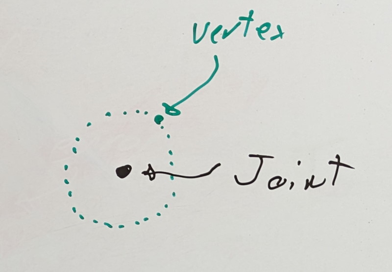
26 Feb 2023As I’ve previously written about, the Animation Compression Library measures the error introduced through compression by approximating the skinning deformation typically done with a graphical mesh. To do so, we define a rigid shell around each joint: a sphere. It is a crude approximation, but the method is otherwise very flexible, and any other shape could be used: a box, convex, etc. This rigid shell is then transformed using its joint transform at every point in time (provided as input through an animation clip). Using only individual joints, this process works in local space of the joint (local space) as transforms are relative to their parent joint in the skeleton hierarchy. When a joint chain that includes the root joint is used, the process works in local space of the object (or object space). While local space only accounts for a single transform (the joint’s), in object space we can account for any number of joints, it depends entirely on the topology of the joint hierarchy. As a result of these extra joints, measuring the error in object space is slower than in local space. Nevertheless, this method is very simple to implement and tune since the resulting error is a 3D displacement between the raw rigid shell and the lossy rigid shell undergoing compression.
ACL leverages this technique and uses it in two ways when optimizing the quantization bit rates (e.g finding how many bits to use for each joint transform).
First, for each joint, we proceed to find the lowest bit rate that meets our specified precision requirement (user provided, per joint). To do so, a pre-generated list of permutations is hardcoded of all possible bit rate combinations for a joint’s rotation, translation, and scale. That list is sorted by total transform size. We then simply iterate on that list in order, testing everything until we meet our precision target. We start with the most lossy bit rates and work our way up, adding more precision as we go along. This is an exhaustive search and to keep it fast, we do this processing in local space of each joint. Once this first pass is done, each joint has an approximate answer for its ideal bit rate. A joint may end up needing more precision to account for object space error (since error accumulates down the joint hierarchy), but it will never need less precision. This thus puts a lower bound on our compressed size.
Second, for each joint chain, we check the error in object space and try multiple permutations by slowly increasing the bit rate on various joints in the chain. This process is much slower and is controlled through the compression level setting which allows a user to tune how much time should be spent by ACL when attempting to optimize for size. Because the first pass only found an approximate answer in local space, this second pass is very important as it enforces our precision requirements in object space by accounting for the full joint hierarchy. Despite aggressive caching, unrolling, and many optimizations, this is by far the slowest part during compression.
This algorithm was implemented years ago, and it works great. But ever since I wrote it, I’ve been thinking of ways to improve it. After all, while it finds a local minimum, there is no guarantee that it is the true global minima which would yield the optimal compressed size. I’ve so far failed to come up with a way to find that optimal minima, but I’ve gotten one step closer!
To the drawing board
Why do we have two passes?
The second pass, in object space, is necessary because it is the one that accounts for the true error as it accumulates throughout the joint hierarchy. However, it is very hard to properly direct because the search space is huge. We need to try multiple bit rate permutations on multiple joint permutations within a chain. How do we pick which bit rate permutations to try? How do we pick which joint permutations to try? If we increase the bit rate towards the root of the hierarchy, we add precision that will improve every child that follows but there is no guarantee that even if we push it to retain full precision that we’ll be able to meet our precision requirements (some clips are exotic). This pass is thus trying to stumble to an acceptable solution and if it fails after spending a tunable amount of time, we give up and bump the bit rates of every joint in the chain as high as we need one by one, greedily. This is far from optimal…
To help it find a solution, it would be best if we could supply it with an initial guess that we hope is close to the ideal solution. The closer this initial guess is to the global minima, the higher our chances will be that we can find it in the second pass. A better guess thus directly leads to a lower memory footprint (the second pass can’t drift as far) and faster compression (the search space is vastly reduced). This is where the first pass comes in. Right off the bat, we know that bit rates that violate our precision requirements in local space will also violate them in object space since our parent joints can only add to our overall error (in practice, the error sometimes compensates but it only does so randomly and thus can’t be relied on). Since testing the error in local space is very fast, we can perform the exhaustive search mentioned above to trim the search space dramatically.
If only we could calculate the object space error using local space information… We can’t, but we can get close!
Long-range attachments
Kim, Tae & Chentanez, Nuttapong & Müller, Matthias. (2012). Long Range Attachments - A Method to Simulate Inextensible Clothing in Computer Games. 305-310. 10.2312/SCA/SCA12/305-310.
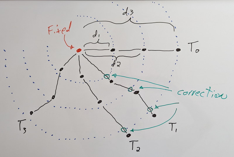
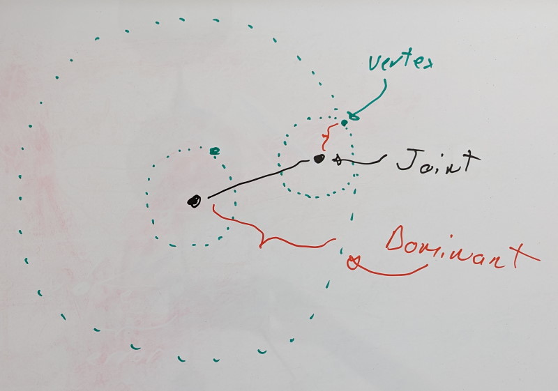
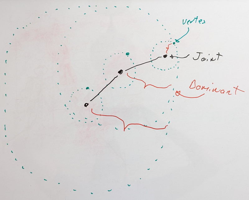
Above: A static vertex in red with 3 attached dynamic vertices in black. A long-range constraint is added for each dynamic vertex, labeled d1, d2, and d3. T0 shows the initial configuration and its evolution over time. When a vertex extends past the long-range constraint, a correction (in green) is applied. Vertices within the limits of the long-range constraints are unaffected.
Back around 2014, I read the above paper on cloth simulation. It describes the concept of long-range attachments to accelerate and improve convergence of distance constraints (e.g. making sure the cloth doesn’t stretch). They start at a fixed point (where the cloth is rigidly attached to something) and they proceed to add additional clamping distance constraints (meaning the distance can be shorter than the desired distance, but no longer) between each simulated vertex on the cloth and the fixed point. These extra constraints help bring back the vertices when the constraints are violated under stress.
A few years later, it struck me: we can use the same general idea when estimating our error!
Dominance based error estimation
When we compress a joint transform, error is introduced. However, the error may or may not be visible to the naked eye. How important the error is depends on one thing: the distance of the rigid shell.
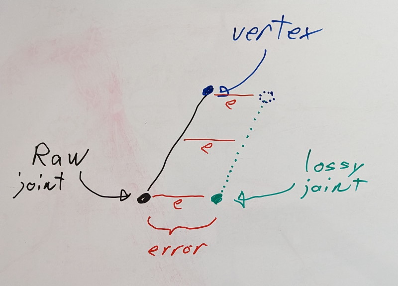
For the translation and scale parts of each transform, the error is independent of the distance of the rigid shell. This means that a 1% error in those, yields a 1% error regardless of how far the rigid shell lives with respect to the joint.
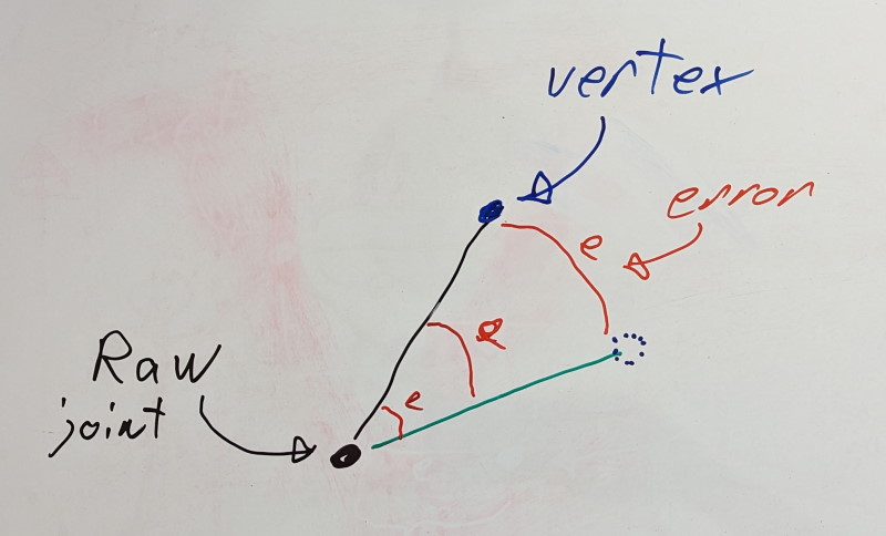
However, the story is different for a transform’s rotation: distance acts as a lever. A 1% error on the rotation does not translate in the same way to the rigid shell. It depends on how close the rigid shell is to the joint. The closer it lives, the lower the error will be and the further it lives, the higher the error.
Using this knowledge, we can reframe our problem. When we measure the error in local space for a joint X, we wish to do so on the furthest rigid shell it can influence. That furthest rigid shell of joint X will be associated with a joint that lives in the same chain. It could be X itself or it could be some child joint Y. We’ll call this joint Y the dominant joint of X.
The dominant rigid shell of a dominant joint is formed through its associated virtual vertex, the dominant vertex.
For leaf joints with no children, we have a single joint in our chain, and it is thus its own dominant joint.
If we add a new joint, we look at it and its immediate children. Are the dominant joints of its children still dominant or is the new joint its own dominant joint? To find it, we look at the rigid shells formed by the dominant vertices of each joint and we pick the furthest.
After all, if we were to measure the error on any rigid shell enclosed within the dominant shell, the error would either be identical (if there is no error contribution from the rotation component) or lower. Distance is king and we wish to look for error as far as we can.
As more joints are introduced, we iterate with the same logic at each joint. Iteration thus starts with leaf joints and proceeds towards the root. You can find the code for this here.
An important part of this process is the step wise nature. By evaluating joints one at a time, we find and update the dominant vertex distance by adding the current vertex distance (the distance between the vertex and its joint). This propagates the geodesic distance. This ensures that even if a joint chain folds on itself, the resulting dominant shell distance is only ever increasing as if every joint was in a straight line.
The last piece of the puzzle is the precision threshold when we measure the error. Because we use the dominant shell as a conservative estimate, we must account for the fact that intermediate joints in a chain will contain some error. Our precision threshold represents an upper bound on the error we’ll allow and a target that we’ll try to reach when optimizing the bit rates. For some bit rate, if the error is above the threshold, we’ll try a lower value, but if it is below the threshold, we’ll try a higher value since we have room to grow. As such, joints in a chain will add their precision threshold to their virtual vertex distance when computing the dominant shell distance except for the dominant joint. The dominant joint’s precision threshold will be used when measuring the error and accounted for there.
This process is done for every keyframe in a clip and the dominant rigid shell is retained for each joint. I also tried to do this processing for each segment ACL works with and there was no measurable impact.
Once computed, ACL then proceeds as before using this new dominant rigid shell distance and the dominant precision threshold. It is used in both passes. Even when measuring a joint in object space, we need to account for its children.
But wait, there’s more!
After implementing this, I realized I could use this trick to fix something else that had been bothering me: constant sub-track collapsing. For each sub-track (rotation, translation, and scale), ACL attempts to determine if they are constant along the whole clip. If they are, we can store a single sample: the reference constant value (12 bytes). This considerably lowers the memory footprint. Furthermore, if this single sample is equal to the default value for that sub-track (either the identity or the bind pose value when stripping the bind pose), the constant sample can be removed as well and reconstructed during decompression. A default sub-track uses only 2 bits!
Until now, ACL used individual precision thresholds for rotation, translation, and scale sub-tracks. This has been a source of frustration for some time. While the error metric uses a single 3D displacement as its precision threshold with intuitive units (e.g. whatever the runtime uses to measure distance), the constant thresholds were this special edge case with non-intuitive units (scale doesn’t even have units). It also meant that ACL was not able to account for the error down the chain: it only looked in local space, not object space. It never occurred to me that I could have leveraged the regular error metric and computed the object space error until I implemented this optimization. Suddenly, it just made sense to use the same trick and skip the object space part altogether: we can use the dominant rigid shell.
This allowed me to remove the constant detection thresholds in favor of the single precision threshold used throughout the rest of the compression. A simpler, leaner API, with less room for user error while improving the resulting accuracy by properly accounting for every joint in a chain.
Show me the money
The results speak for themselves:
Baseline:
| Data Set | Compressed Size | Compression Speed | Error 99th percentile |
|---|---|---|---|
| CMU | 72.14 MB | 13055.47 KB/sec | 0.0089 cm |
| Paragon | 208.72 MB | 10243.11 KB/sec | 0.0098 cm |
| Matinee Fight | 8.18 MB | 16419.63 KB/sec | 0.0201 cm |
With dominant rigid shells:
| Data Set | Compressed Size | Compression Speed | Error 99th percentile |
|---|---|---|---|
| CMU | 65.83 MB (-8.7%) | 34682.23 KB/sec (2.7x) | 0.0088 cm |
| Paragon | 184.41 MB (-11.6%) | 20858.25 KB/sec (2.0x) | 0.0088 cm |
| Matinee Fight | 8.11 MB (-0.9%) | 17097.23 KB/sec (1.0x) | 0.0092 cm |
The memory footprint reduces by over 10% in some data sets and compression is twice as fast (the median compression time per clip for Paragon is now 11 milliseconds)! Gains like this are hard to come by now that ACL has been so heavily optimized already; this is really significant. This optimization maintains the same great accuracy with no impact whatsoever to decompression performance.
The memory footprint reduces because our initial guess following the first pass is now much better: it accounts for the potential error of any children. This leaves less room for drifting off course in the second pass. And with our improved guess, the search space is considerably reduced leading to much faster convergence.
Now that this optimization has landed in ACL develop, I am getting close to finishing up the upcoming ACL 2.1 release which will include it and much more. Stay tuned!