16 Dec 2023
After over 30 months of work, the Animation Compression Library has finally reached v2.1 along with an updated v2.1 Unreal Engine plugin.
Notable changes in this release include:
Overall, memory savings average between 10-15% for this release compared to the prior version. Decompression performance remained largely the same if not slightly faster. Compression is slightly slower in part due to the default compression level being more aggressive thanks to many performance improvements that make it viable. Visual fidelity improved slightly as well.
This release took much longer than prior releases because a lot of time was spent on quality-of-life improvements. CI now runs regression tests and tests more platforms and toolchains. CI uses docker which makes finding and fixing regressions much easier. A satellite project was spun off to generate the regression test data. Together, these changes make it much faster for me to polish, test, and finalize a release.
This release saw many contributions from the community through GitHub issues, questions, code, and fixes. Special thanks to all ACL contributors!
Who uses ACL?
The Unreal Engine plugin of ACL has proved to be quite popular over the years. The reverse engineering community over at Gildor’s Forums have a post that tracks who uses ACL in UE. At the time of writing, the list includes:
Desktop games:
All latest Dontnod’s games: two last episodes of Life is Strange 2, Twin Mirror, Tell Me Why, most likely all their future releases as well.
Beyond a Steel Sky, Chivalry 2, Fortnite (current version), Kena: Bridge of Spirits, Remnant: From the Ashes (current version), Rogue Company (current version), Star Wars: Tales From The Galaxy’s Edge, Final Fantasy VII Remake (including Intergrade), The Ascent, The Dark Pictures Anthology (Man of Medan / Little Hope / House of Ashes / Devil in Me) (current version), Valorant, Evil Dead: The Game, The Quarry, The DioField Chronicle, Borderlands 3, Tiny Tina’s Wonderlands, Medieval Dynasty (current version), Divine Knockout, Lost Ark, SD Gundam Battle Alliance, Back 4 Blood, KartRider: Drift (current version), Dragon Quest X Offline, Gran Saga (current version), Gundam Evolution (current version), The Outlast Trials, Harvestella, Valkyrie Elysium, The Dark Pictures Anthology: The Devil In Me, The Callisto Protocol, Synced (current version), High On Life, PlayerUnknown’s Battlegrounds (current version), Deliver Us Mars, Sherlock Holmes The Awakened, Hogwarts Legacy, Wanted: Dead, Like a Dragon: Ishin, Atomic Heart, Crime Boss: Rockay City, Dead Island 2, Star Wars Jedi: Survivor, Redfall, Park Beyond, The Lord of the Rings: Gollum, Gangstar NY, Lies of P, Warhaven (current version), AEW: Fight Forever, Legend of the Condor, Crossfire: Sierra Squad, Mortal Kombat 1, My Hero Ultra Rumble, Battle Crush, Overkill’s The Walking Dead, Payday 3
Mobile games:
Apex Legends Mobile (current version), Dislyte, Marvel Future Revolution, Mir4, Ni no Kuni: Cross Worlds, PUBG Mobile (current version), Undecember, Blade & Soul Revolution (current version), Crystal of Atlan, Mortal Kombat: Onslaught (old versions), Farlight 84, ArcheAge War, Assassin’s Creed: Codename Jade, Undawn, Arena Breakout, High Energy Heroes, Dream Star
Console games:
No More Heroes 3
Many others use ACL in their own internal game engines. If you aren’t using it yet, let me know if anything is missing!
What’s next
I’ve already started fleshing out the task list for the next minor release here. This release will bring about more memory footprint improvements.
If you use ACL and would like to help prioritize the work I do, feel free to reach out and provide feedback or requests!
Now that ACL is the default codec in Unreal Engine 5.3, this reduces my maintenance burden considerably as Epic has taken over the plugin development. This will leave me to focus on improving the standalone ACL project and Realtime Math. Going forward, I will aim for smaller and more frequent releases.
17 Sep 2023
The very first release of the Animation Compression Library (ACL) Unreal Engine plugin came out in July of 2018 and required custom engine changes. It was a bit rough around the edges. Still, in the releases that followed, despite the integration hurdles, it slowly grew in popularity in games large and small. Two years later, version 1.0 came out with official support of UE 4.25 through the Unreal Engine Marketplace. Offering backwards compatibility with each new release and a solid alternative to the stock engine codecs, the plugin continued to grow in popularity. Today, many of the most demanding and popular console and mobile games that use Unreal already use ACL (Fortnite itself has been using it for many years). It is thus with great pleasure that I can announce that as of UE 5.3, the ACL plugin comes out of the box with batteries included as the default animation compression codec!
This represents the culmination of many years of hard work and slow but steady progress. This new chapter is very exciting for a few reasons:
- Better quality, compression and decompression performance for all UE users out of the box.
- A dramatically smaller memory footprint: ACL saves over 30% compared with the defaults codecs in UE 5.2 and more savings will come with the next ACL 2.1 release later this year (up to 46% smaller than UE 5.2).
- Maintenance churn to keep up with each UE release was a significant burden. Epic will now take ownership of the plugin by continuing its development in their fork as part of the main Unreal Engine development branch.
- With official UE distribution comes better documentation, localization, and support through the Unreal Developer Network (UDN). This means a reduced burden for me as I now can support the plugin as part of my day job at Epic as opposed to doing so on my personal time (burning that midnight oil).
Best of all, by no longer having to maintain the plugin in my spare time, it will allow me to better focus on the core of ACL that benefits everyone. Many proprietary game engines leverage standalone ACL and in fact quite a few code contributions (and ideas) over the years came from them.
Unfortunately, it does mean that some tradeoffs had to be made:
- The GitHub version of the plugin will remain largely in read only mode, taking in only critical bug fixes. It will retain its current MIT License. Contributions should instead be directed to the Unreal Engine version of the plugin.
- The Unreal Engine Marketplace version of the plugin will no longer be updated to keep up with each UE release (since it comes packaged with the engine already).
- Any changes to the plugin will not be backwards compatible as they will be made in the Unreal Engine main development branch. To get the latest improvements, you’ll have to update your engine version (like any other built in feature).
- Each plugin release will no longer publish statistics comparing ACL to the other UE codecs.
- The ACL plugin within UE will take on the engine code license (it already had a dual license like all code plugins do on the Unreal Engine Marketplace).
That being said, once ACL 2.1 comes out later this year, one last release of the plugin will be published on GitHub and the Unreal Engine Marketplace (for UE versions before 5.3). It brings many improvements to the memory footprint and visual fidelity. A future version of UE will include it (TBD).
To further clarify, the core ACL project will remain with me and continue to evolve on GitHub with the MIT License as it always has. I still have a long list of improvements and research topics to explore!
26 Feb 2023
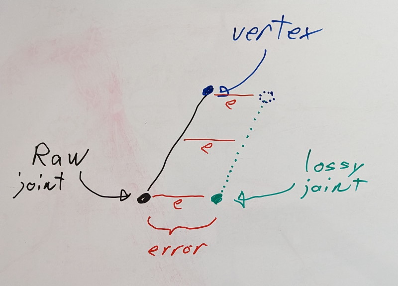
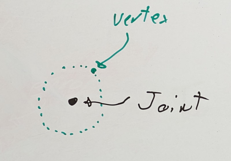
As I’ve previously written about, the Animation Compression Library measures the error introduced through compression by approximating the skinning deformation typically done with a graphical mesh. To do so, we define a rigid shell around each joint: a sphere. It is a crude approximation, but the method is otherwise very flexible, and any other shape could be used: a box, convex, etc. This rigid shell is then transformed using its joint transform at every point in time (provided as input through an animation clip). Using only individual joints, this process works in local space of the joint (local space) as transforms are relative to their parent joint in the skeleton hierarchy. When a joint chain that includes the root joint is used, the process works in local space of the object (or object space). While local space only accounts for a single transform (the joint’s), in object space we can account for any number of joints, it depends entirely on the topology of the joint hierarchy. As a result of these extra joints, measuring the error in object space is slower than in local space. Nevertheless, this method is very simple to implement and tune since the resulting error is a 3D displacement between the raw rigid shell and the lossy rigid shell undergoing compression.
ACL leverages this technique and uses it in two ways when optimizing the quantization bit rates (e.g finding how many bits to use for each joint transform).
First, for each joint, we proceed to find the lowest bit rate that meets our specified precision requirement (user provided, per joint). To do so, a pre-generated list of permutations is hardcoded of all possible bit rate combinations for a joint’s rotation, translation, and scale. That list is sorted by total transform size. We then simply iterate on that list in order, testing everything until we meet our precision target. We start with the most lossy bit rates and work our way up, adding more precision as we go along. This is an exhaustive search and to keep it fast, we do this processing in local space of each joint. Once this first pass is done, each joint has an approximate answer for its ideal bit rate. A joint may end up needing more precision to account for object space error (since error accumulates down the joint hierarchy), but it will never need less precision. This thus puts a lower bound on our compressed size.
Second, for each joint chain, we check the error in object space and try multiple permutations by slowly increasing the bit rate on various joints in the chain. This process is much slower and is controlled through the compression level setting which allows a user to tune how much time should be spent by ACL when attempting to optimize for size. Because the first pass only found an approximate answer in local space, this second pass is very important as it enforces our precision requirements in object space by accounting for the full joint hierarchy. Despite aggressive caching, unrolling, and many optimizations, this is by far the slowest part during compression.
This algorithm was implemented years ago, and it works great. But ever since I wrote it, I’ve been thinking of ways to improve it. After all, while it finds a local minimum, there is no guarantee that it is the true global minima which would yield the optimal compressed size. I’ve so far failed to come up with a way to find that optimal minima, but I’ve gotten one step closer!
To the drawing board
Why do we have two passes?
The second pass, in object space, is necessary because it is the one that accounts for the true error as it accumulates throughout the joint hierarchy. However, it is very hard to properly direct because the search space is huge. We need to try multiple bit rate permutations on multiple joint permutations within a chain. How do we pick which bit rate permutations to try? How do we pick which joint permutations to try? If we increase the bit rate towards the root of the hierarchy, we add precision that will improve every child that follows but there is no guarantee that even if we push it to retain full precision that we’ll be able to meet our precision requirements (some clips are exotic). This pass is thus trying to stumble to an acceptable solution and if it fails after spending a tunable amount of time, we give up and bump the bit rates of every joint in the chain as high as we need one by one, greedily. This is far from optimal…
To help it find a solution, it would be best if we could supply it with an initial guess that we hope is close to the ideal solution. The closer this initial guess is to the global minima, the higher our chances will be that we can find it in the second pass. A better guess thus directly leads to a lower memory footprint (the second pass can’t drift as far) and faster compression (the search space is vastly reduced). This is where the first pass comes in. Right off the bat, we know that bit rates that violate our precision requirements in local space will also violate them in object space since our parent joints can only add to our overall error (in practice, the error sometimes compensates but it only does so randomly and thus can’t be relied on). Since testing the error in local space is very fast, we can perform the exhaustive search mentioned above to trim the search space dramatically.
If only we could calculate the object space error using local space information… We can’t, but we can get close!
Long-range attachments
Kim, Tae & Chentanez, Nuttapong & Müller, Matthias. (2012). Long Range Attachments - A Method to Simulate Inextensible Clothing in Computer Games. 305-310. 10.2312/SCA/SCA12/305-310.

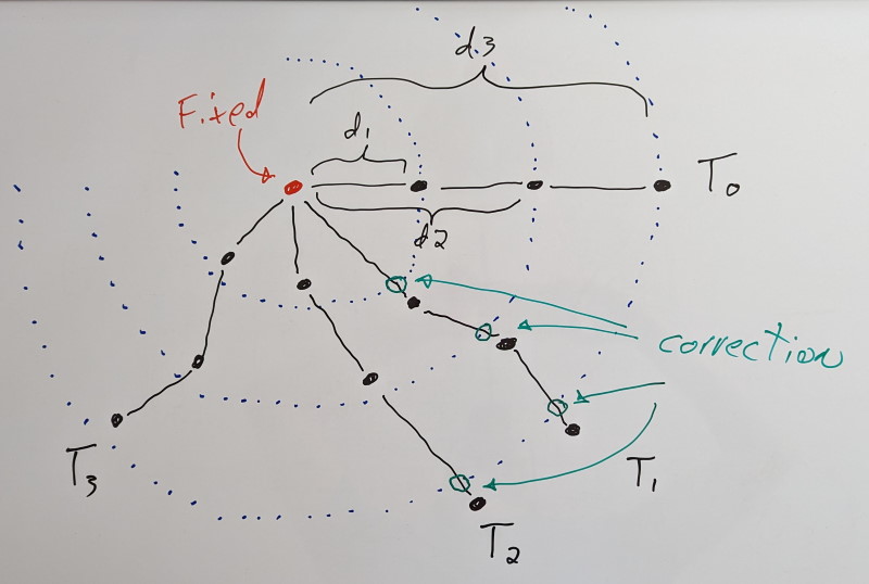
Above: A static vertex in red with 3 attached dynamic vertices in black. A long-range constraint is added for each dynamic vertex, labeled d1, d2, and d3. T0 shows the initial configuration and its evolution over time. When a vertex extends past the long-range constraint, a correction (in green) is applied. Vertices within the limits of the long-range constraints are unaffected.
Back around 2014, I read the above paper on cloth simulation. It describes the concept of long-range attachments to accelerate and improve convergence of distance constraints (e.g. making sure the cloth doesn’t stretch). They start at a fixed point (where the cloth is rigidly attached to something) and they proceed to add additional clamping distance constraints (meaning the distance can be shorter than the desired distance, but no longer) between each simulated vertex on the cloth and the fixed point. These extra constraints help bring back the vertices when the constraints are violated under stress.
A few years later, it struck me: we can use the same general idea when estimating our error!
Dominance based error estimation
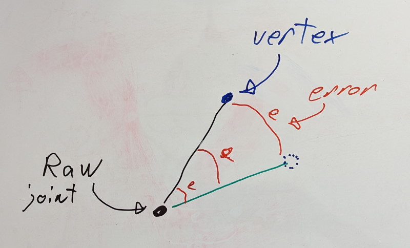
When we compress a joint transform, error is introduced. However, the error may or may not be visible to the naked eye. How important the error is depends on one thing: the distance of the rigid shell.

For the translation and scale parts of each transform, the error is independent of the distance of the rigid shell. This means that a 1% error in those, yields a 1% error regardless of how far the rigid shell lives with respect to the joint.

However, the story is different for a transform’s rotation: distance acts as a lever. A 1% error on the rotation does not translate in the same way to the rigid shell. It depends on how close the rigid shell is to the joint. The closer it lives, the lower the error will be and the further it lives, the higher the error.
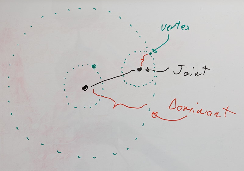
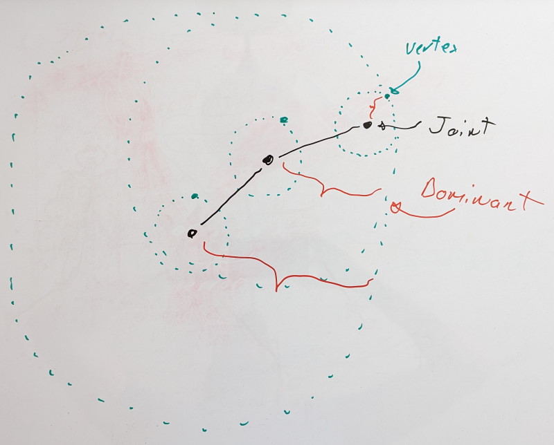
Using this knowledge, we can reframe our problem. When we measure the error in local space for a joint X, we wish to do so on the furthest rigid shell it can influence. That furthest rigid shell of joint X will be associated with a joint that lives in the same chain. It could be X itself or it could be some child joint Y. We’ll call this joint Y the dominant joint of X.
The dominant rigid shell of a dominant joint is formed through its associated virtual vertex, the dominant vertex.

For leaf joints with no children, we have a single joint in our chain, and it is thus its own dominant joint.

If we add a new joint, we look at it and its immediate children. Are the dominant joints of its children still dominant or is the new joint its own dominant joint? To find it, we look at the rigid shells formed by the dominant vertices of each joint and we pick the furthest.
After all, if we were to measure the error on any rigid shell enclosed within the dominant shell, the error would either be identical (if there is no error contribution from the rotation component) or lower. Distance is king and we wish to look for error as far as we can.

As more joints are introduced, we iterate with the same logic at each joint. Iteration thus starts with leaf joints and proceeds towards the root. You can find the code for this here.
An important part of this process is the step wise nature. By evaluating joints one at a time, we find and update the dominant vertex distance by adding the current vertex distance (the distance between the vertex and its joint). This propagates the geodesic distance. This ensures that even if a joint chain folds on itself, the resulting dominant shell distance is only ever increasing as if every joint was in a straight line.
The last piece of the puzzle is the precision threshold when we measure the error. Because we use the dominant shell as a conservative estimate, we must account for the fact that intermediate joints in a chain will contain some error. Our precision threshold represents an upper bound on the error we’ll allow and a target that we’ll try to reach when optimizing the bit rates. For some bit rate, if the error is above the threshold, we’ll try a lower value, but if it is below the threshold, we’ll try a higher value since we have room to grow. As such, joints in a chain will add their precision threshold to their virtual vertex distance when computing the dominant shell distance except for the dominant joint. The dominant joint’s precision threshold will be used when measuring the error and accounted for there.
This process is done for every keyframe in a clip and the dominant rigid shell is retained for each joint. I also tried to do this processing for each segment ACL works with and there was no measurable impact.
Once computed, ACL then proceeds as before using this new dominant rigid shell distance and the dominant precision threshold. It is used in both passes. Even when measuring a joint in object space, we need to account for its children.
But wait, there’s more!
After implementing this, I realized I could use this trick to fix something else that had been bothering me: constant sub-track collapsing. For each sub-track (rotation, translation, and scale), ACL attempts to determine if they are constant along the whole clip. If they are, we can store a single sample: the reference constant value (12 bytes). This considerably lowers the memory footprint. Furthermore, if this single sample is equal to the default value for that sub-track (either the identity or the bind pose value when stripping the bind pose), the constant sample can be removed as well and reconstructed during decompression. A default sub-track uses only 2 bits!
Until now, ACL used individual precision thresholds for rotation, translation, and scale sub-tracks. This has been a source of frustration for some time. While the error metric uses a single 3D displacement as its precision threshold with intuitive units (e.g. whatever the runtime uses to measure distance), the constant thresholds were this special edge case with non-intuitive units (scale doesn’t even have units). It also meant that ACL was not able to account for the error down the chain: it only looked in local space, not object space. It never occurred to me that I could have leveraged the regular error metric and computed the object space error until I implemented this optimization. Suddenly, it just made sense to use the same trick and skip the object space part altogether: we can use the dominant rigid shell.
This allowed me to remove the constant detection thresholds in favor of the single precision threshold used throughout the rest of the compression. A simpler, leaner API, with less room for user error while improving the resulting accuracy by properly accounting for every joint in a chain.
Show me the money
The results speak for themselves:
Baseline:
| Data Set |
Compressed Size |
Compression Speed |
Error 99th percentile |
| CMU |
72.14 MB |
13055.47 KB/sec |
0.0089 cm |
| Paragon |
208.72 MB |
10243.11 KB/sec |
0.0098 cm |
| Matinee Fight |
8.18 MB |
16419.63 KB/sec |
0.0201 cm |
With dominant rigid shells:
| Data Set |
Compressed Size |
Compression Speed |
Error 99th percentile |
| CMU |
65.83 MB (-8.7%) |
34682.23 KB/sec (2.7x) |
0.0088 cm |
| Paragon |
184.41 MB (-11.6%) |
20858.25 KB/sec (2.0x) |
0.0088 cm |
| Matinee Fight |
8.11 MB (-0.9%) |
17097.23 KB/sec (1.0x) |
0.0092 cm |
The memory footprint reduces by over 10% in some data sets and compression is twice as fast (the median compression time per clip for Paragon is now 11 milliseconds)! Gains like this are hard to come by now that ACL has been so heavily optimized already; this is really significant. This optimization maintains the same great accuracy with no impact whatsoever to decompression performance.
The memory footprint reduces because our initial guess following the first pass is now much better: it accounts for the potential error of any children. This leaves less room for drifting off course in the second pass. And with our improved guess, the search space is considerably reduced leading to much faster convergence.
Now that this optimization has landed in ACL develop, I am getting close to finishing up the upcoming ACL 2.1 release which will include it and much more. Stay tuned!
Back to table of contents
05 Jun 2022
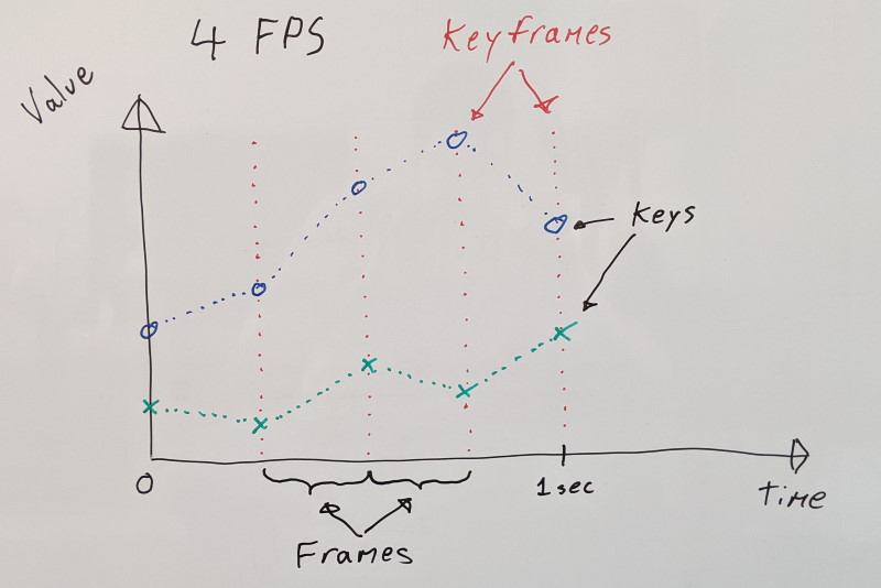
The Animation Compression Library works with uniformly sampled animation clips. For each animated data track, every sample falls at a predictable and regular rate (e.g. 30 samples/frames per second). This is done to keep the decompression code simple and fast: with samples being so regular, they can be packed efficiently, sorted by their timestamp.

When we decompress, we simply find the surrounding samples to reconstruct the value we need.
float t = ... // At what time in the clip we sample

float duration = (num_samples - 1) * sample_rate;
float normalized_t = t / duration;
float sample_offset = normalized_t * (num_samples - 1);

int first_sample = trunc(sample_offset);
int second_sample = min(first_sample + 1, num_samples - 1);

float interpolation_alpha = sample_offset - first_sample;

interpolation_alpha = apply_rounding(interpolation_alpha, rounding_mode);

float result = lerp(sample_values[first_sample], sample_values[second_sample], interpolation_alpha);
This allows us to continously animate every value smoothly over time. However, that is not always necessary or desired. To support these use cases, ACL supports several sample time rounding modes in order to achieve various effects.
Rounding modes:
none: no rounding means that we linearly interpolate.floor: the first/earliest sample is returned with full weight (interpolation alpha = 0.0). This can be used to step animations forward. Visually, on a character animation, it would look like a stop motion performance.ceil: the second/latest sample is returned with full weight (interpolation alpha = 1.0). This might not have a valid use case but ACL supports it regardless for the sake of completeness. Unlike floor above, ceil returns values that are in the future which might not line up with other events that haven’t happened yet: particle effects, audio cues (e.g. footstep sounds), and other animations. If you know of a valid use case for this, please reach out!nearest: the nearest sample is returned with full weight (interpolation alpha = 0.0 or 1.0 using round to nearest). ACL uses this internally when measuring the compression error. The error is measured at every keyframe and because of floating point rounding, we need to ensure that a whole sample is used. Otherwise, we might over/undershoot.per_track: each animated track can specify which rounding mode it wishes to use.
Per track rounding
This is a new feature that has been requested by a few studios (included in the upcoming ACL 2.1 release).
When working with animated data, sometimes tracks within a clip are not homogenous and represent very different things. Synthetic joints can be introduced which do not represent something directly observable (e.g. camera, IK targets, pre-processed data). At times, these do not represent values that can be safely interpolated.
For example, imagine that we wish to animate a stop motion character along with a camera track in a single clip. We wish for the character joints to step forward in time and not interpolate (floor rounding) but the camera must move smoothly and interpolate (no rounding).
More commonly, this happens with scalar tracks. These are often used for animating blend shape (aka morph target) weights along with various other gameplay values. Gameplay tracks can mean anything and even though they are best stored as floating point values (to keep storage and their manipulation simple), they might not represent a smooth range (e.g. integral values, enums, etc).
When such mixing is used, each track can specify what rounding mode to use during decompression (ACL does not store this information in the compressed data).
Note: tracks that do not interpolate smoothly also do not blend smoothly (between multiple clips) and special care must be taken when doing so.
See here for details on how to use this new feature.
During decompression, ACL always interpolates between two samples even if the per track rounding feature is disabled during compilation. The most common rounding mode is none which means we interpolate. This allows us to keep the code simple. We simply snap the interpolation alpha to 0.0 or 1.0 when we floor and ceil respectively (or with nearest) and we make sure to use a stable linear interpolation function.
As a result, every rounding mode has the same performance with the exception of the per track one.
Per track rounding is disabled by default and the code is entirely stripped out because it isn’t commonly required. When enabled, it adds a small amount of overhead on the order of 2-10% slower (AMD Zen2 with SSE2) regardless of which rounding mode individual tracks use.
During decompression, ACL unpacks 8 samples at a time and interpolates them in pairs. These are then cached in a structure on the execution stack. This is done ahead, before the interpolated samples are needed to be written out which means that during interpolation, it does not know which sample belongs to which track. That determination is only done when we read it from the cached structure. The reason for this will be the subject of a future blog post but it is done to speed up decompression by hiding memory latency.
As a result of this design decision, the only way to support per track rounding is to cache all possible rounding results. When we need to read an interpolated sample, we can simply index into the cache with the rounding mode chosen for that specific track. In practice, this is much cheaper than it sounds because even though it adds quite a few extra instructions to execute (SSE2 will be quite a bit worse than AVX here due to the lack of VEX prefix and blend instructions), they can do so independently of other surrounding instructions and in the shadow of expensive square root instructions for rotation sub-tracks (we need to reconstruct the quaternion w component and we need to normalize the resulting interpolated value). In practice, we don’t have to interpolate three times (one for each possible alpha value) because both 0.0 and 1.0 are trivial.
Caveats when key frames are removed
When the database feature is used, things get a bit more complicated. Whole keyframes can be moved to the database and optionally stripped. This means that non-neighboring keyframes might interpolate together.
When all tracks interpolate with the same rounding mode, we can reconstruct the right interpolation alpha to use based on our closest keyframes present.
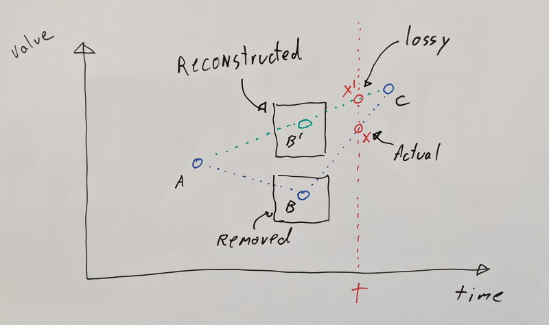
For example, let’s say that we have 3 keyframes: A, B, and C. Consider the case where we sample the time just after where B lies (at time t).

If B has been moved to the database and isn’t present in memory during decompression, we have to reconstruct our value based on our closest remaining neighbors A and C (an inherently lossy process). When all tracks use the same rounding mode, this is clean and fast since only one interpolation alpha is needed for all tracks:
none: one alpha value is needed between A and C, past the 50% mark where B lies (see x' above)floor: one alpha value is needed at 50% between A and C to reconstruct B (see B' above)ceil: one alpha value is needed at 100% on Cnearest: the same alpha value as floor and ceil is used
However, consider what happens when individual tracks have their own rounding mode. We need three different interpolation alphas that are not trivial (0.0 or 1.0). Trivial alphas are very cheap since they fully match our known samples. To keep the code flexible and fast during decompression, we would have to fully interpolate three times:
- Once for
floor since the interpolation alpha needed for it might not be a nice number like 0.5 if multiple consecutive keyframes have been removed.
- Once for
ceil for the same reason as floor.
- Once for
none for our actual interpolated value.
As a result, the behavior will differ for the time being as ACL will return A with floor instead of the reconstructed B. This is unfortunate and I hope to address this in the next minor release (v2.2).
Note: This discrepancy will only happen when interpolating with missing keyframes. If the missing keyframes are streamed in, everything will work as expected as if no database was used.
In a future release, ACL will support splitting tracks into layers to group them together. This will allow us to use different rounding modes for different layers. We will also be able to specify which tracks have values that can be interpolated or not, allowing us to identify boundary keyframes that cannot be moved to the database.
I would have liked to properly handle this right off the bat however due to time constraints, I opted to defer this work until the next release. I’m hoping to finalize the release of v2.1 this year. There is no ETA yet for v2.2 but it will focus on streaming and other improvements.
Back to table of contents
03 Apr 2022
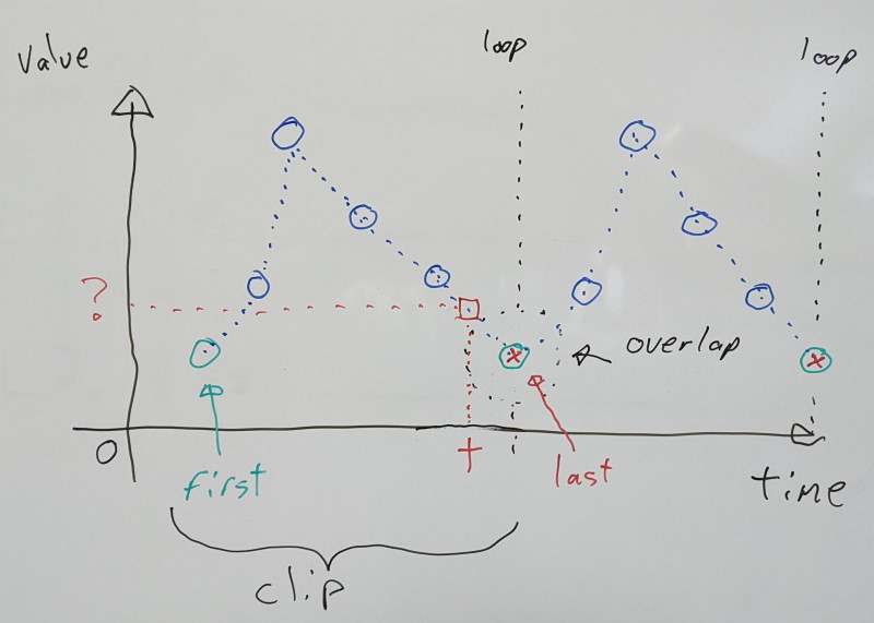
Animations that loop have a unique property in that the last character pose must exactly match the first, for playback to be seamless as they wrap around. As a result, this means that the repeating first/last pose is redundant. Looping animations are fairly common, and it thus makes sense to try and leverage this in order to reduce the memory footprint. However, there are important caveats with this, and special care must be taken.
The Animation Compression Library now supports two looping modes: clamp and wrap.
To illustrate things, I will use a simple 1D repeating sequence but in practice, everything can be generalized in 3D (e.g. translations), 4D (e.g. rotation quaternions), and other dimensions.
Clamping loops
Clamping requires the first and last samples to match exactly, and both will be retained in the final compressed data. This keeps things very simple.

Calculating the clip duration can be achieved by taking the number of samples and subtracting one before multiplying by the sampling rate (e.g. 30 FPS). We subtract by one because we count how many intervals of time we have in between our samples.
If we wish to sample the clip at some time t, we normalize it by dividing by the clip duration to bring the resulting value between [0.0, 1.0] inclusive.
We can then multiply it with the last sample index to find which two values to use when interpolating:
- The first sample is the
floor value (or the truncated value)
- The second sample is the
ceil value (or simply the first + 1) we clamp with the last sample index
The interpolation alpha value between the two is the resulting fractional part.
Reconstructing our desired value can then be achieved by interpolating the two samples.
float duration = (num_samples - 1) * sample_rate;
float normalized_t = t / duration;
float sample_offset = normalized_t * (num_samples - 1);

int first_sample = trunc(sample_offset);
int second_sample = min(first_sample + 1, num_samples - 1);

float interpolation_alpha = sample_offset - first_sample;

float result = lerp(sample_values[first_sample], sample_values[second_sample], interpolation_alpha);
This works for any sequence with at least one sample, regardless of whether or not it loops. By design, we never interpolate between the first and last samples as playback loops around.
This is the behavior in ACL v2.0 and prior. No effort had been made to take advantage of looping animations.
Wrapping loops
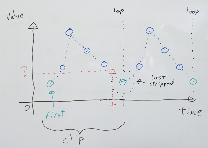
Wrapping strips the last sample, and instead uses the first sample to interpolate with. As a result, unlike with the clamp mode, it will interpolate between the first and last samples as playback loops around.

This complicates things because it means that the duration of our clip is no longer a function of the number of samples actually present. One less sample is stored, but we have to remember to account for our repeating first sample.
Accounting for that fact, this gives us the following:
float duration = num_samples * sample_rate;
float normalized_t = t / duration;
float sample_offset = normalized_t * num_samples;

int first_sample = trunc(sample_offset);
int second_sample = first_sample + 1;

if (first_sample == num_samples) {
    // Sampling the last sample with full weight, use the first sample
    first_sample = second_sample = 0;
    sample_offset = 0.0f;
}
else if (second_sample == num_samples) {
    // Interpolating with the last sample, use the first sample
    second_sample = 0;
}

float interpolation_alpha = sample_offset - first_sample;

float result = lerp(sample_values[first_sample], sample_values[second_sample], interpolation_alpha);
By design, the above logic only works for clips which have had their last sample removed. As such, it is not suitable for non-looping clips.
How much memory does it save?
I analyzed the animation clips from Paragon to see how much memory a single key frame (whole pose at a point in time) uses. The results were somewhat underwhelming to say the least.
| Paragon |
Before |
After |
| Compressed size |
208.93 MB |
208.71 MB |
| Track error 99th percentile |
0.0099 cm |
0.0099 cm |
Roughly 200 KB were saved or about 0.1% even though 1454 clips (out of 6558) were identified as looping. Looking deeper into the data shows the following hard truth: animated key frame data is pretty small to begin with.
| Paragon |
50th percentile |
85th percentile |
99th percentile |
| Animated frame size |
146.62 Bytes |
328.88 Bytes |
756.38 Bytes |
Half the clips have an animated key frame size of 146 bytes or smaller. Because joints are not all animated, they do not all benefit equally.
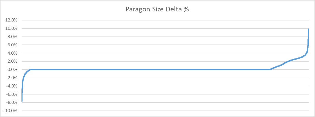
Here is the full distribution of how much memory was saved as a percentage of the original size:

Interestingly, some clips end up larger when the last key frame is removed. How come? It all boils down to the fact that ACL tries to split the number of key frames evenly across all sub-segments it generates. Segments are used to improve accuracy and lower the memory footprint but the current method is naive and will be improved on in the future. As such, when a loop is detected, ACL can do one of two things: the last key frame can be removed before segments are created or afterwards. I opted to do so before to ensure proper balancing. As such, through the re-balancing that occurs, some clips can end up being larger. Either way, the small size of the animated key frame data puts a fairly low ceiling on how much this optimization can save.
Side node: thanks to this, I found a small bug that impacts a very small subset of clips. Clips impacted by this ended up with segments containing more key frames than they otherwise would have resulting in a slightly larger memory footprint.
Caveats
Special care must be taken when removing the last sample, as joint tracks are not all equal. In a looping clip, the last sample will match the first for joints which have a direct impact on visual feedback to the user, but it might not be the case for joints which have an indirect impact, or those that have no impact. For example, while the joint for a character’s hand has direct visual feedback as we see it on screen, other joints like the root have only indirect feedback (through root motion), and any number of custom invisible joints might exist for things like inverse kinematics and other metadata required.
A looping clip with root motion might have a perfectly matching last sample for the visible portion of the character pose, but the root value might differ between the two. When this is the case, removing the last sample means truncating important data! For that reason, ACL only detects wrapping when ALL joints repeat perfectly between their first and last sample.
Why is root motion special?
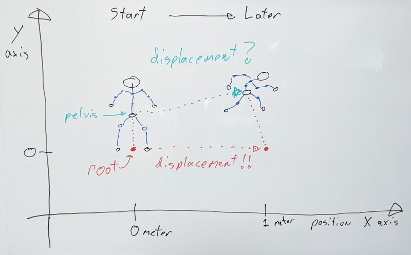
An animation clip contains a series of transforms for every joint at different points in time. To remove as much redundancy as possible, joints are stored relative to their parent (if they have one, local space). In order to display the visual mesh, each joint transform is combined with its parent, recursively, all the way to the root of the character (converting from local space to object space).
In an animation editor, a character will be animated relative to some origin point at [0,0,0] (object space). However, in practice, we need to be able to play that animation anywhere in the world (world space). As such, we need to transform joints from object space into world space by using the character’s transform.

The pelvis joint is usually the highest most visible joint in the hierarchy with the legs and spine in turn parented to it, etc. When the character moves, every joint has direct visual feedback as their movement deforms the parts of the visual mesh attached to them (through the rigid skinning process).
Now what happens if we wish to make a walking animation where the character moves at some desired speed? If the pelvis joint is the highest most joint in the hierarchy, this motion will happen there, and it will drag every joint parented to it (because children transforms are stored relative to their parent to avoid having redundant motion in every joint).
This is problematic because now, the character motion is mixed in with what the pelvis does in this particular clip (e.g. swaying back and forth). It is no longer possible to extract cleanly that motion free from the noise of the animation. As the animation plays back in the world, things might be attached to the character (e.g. camera) that we wish to attach to the character himself, and not some particular joint. If only the joints move, this won’t work. As such, we often want to extract this character motion and apply it as a delta from the previous animation update. We would remove this motion from the joints, and instead transfer it onto the character.

To simplify this process, character motion is generally stored in a root joint that sits highest in the joint hierarchy. This joint does not directly move anything, and we instead extract the character motion from it and apply it onto the character.
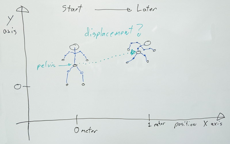
As a result, character motion is stored as an absolute displacement value relative to that [0,0,0] origin mentioned earlier. In a 1-second-long animation where the character moves 1 meter, on the first sample the root value will be zero meters and on the last sample, the value is 1 meter. Values in between can vary depending on how the character velocity changes. As such, even if the character pose is identical between the first and last samples, their root joints differ and CANNOT be interpolated between.
When we sample the animation, we can find out our character motion delta as follow: current_root_position - previous_root_position. This gives us how much the character moved since the last update. When the animation loops, we must break this calculation down into two parts:
last_root_position - previous_root_position to get the trailing end of the motioncurrent_root_position - first_root_position to get the rest of the motion (note that first_root_position is usually zero and can be omitted)
There is also one more special case to consider: if the animation loops more than once since the last update. This can happen for any number of reasons: playback rate changes, the character was off screen for a while and is now visible and updating again, etc. When this happens, we must extract the total displacement of the animation and multiply it by how many times we looped through. The total displacement value lives in our last sample and can simply be read from there: last_root_position * num_loops.
If, for whatever reason, we forcibly remove the last sample, we will no longer have information on how fast the root was moving as it wrapped around. This velocity information is permanently lost and cannot be reconstructed.
It is generally desirable to keep the number of samples for every joints the same for compression purposes within an animation clip. If we don’t, we would need to either store how many samples we have per joints (and there can be many) or whether the last sample has been removed or not. This added overhead and complexity is ideally one we’d like to do without.
It is thus tempting to remove the last sample and estimate the missing value somehow. While this might work with few to no visible artifacts, it can have subtle implications when other things that should be moving at the same overall rate are visible on screen. For example, two characters might be running side by side at the same velocity, but with different animations. Just because the overall velocity is the same (e.g. both move at 1 meter per second), it does not mean that the velocity on the last sample matches. One animation might start fast and slow down before looping, while the other does the opposite. If this is the case, both characters will end up slowly drifting from each other even though they should not.
Back to table of contents
