Animation Compression: Advanced Quantization
12 Mar 2017I first spoke about this technique at the Game Developers Conference (GDC) in 2017 and the slides for that presentation can be found here. The idea is to take everything that is good about simple quantization and super charge it. Since simple quantization is generally a foundation for the other algorithms, this new variant can be used just as well for the same purpose.
It is worth noting that the algorithm I presented used uniform segmenting as well as range reduction both per clip and per block.
The key insight is that with simple quantization, using a hard coded bit rate is very naive and overly simplistic. We can do better, here’s how!
Variable Bit Rate
In the real world, the nature of the data can change quite dramatically from clip to clip, track to track, or even within a track through time. It is thus important to have a solution that can properly adapt to ever changing environmental conditions. A variable bit rate solves this problem for us.
It is ideal for our hierarchical data. As previously mentioned, our bone track data is stored in local space of their parent bone. This means that each bone incurs a small amount of error as a result of the lossy compression and this error will accumulate as we go down the hierarchy. The error accumulates because we need our final bone transforms in world space to perform skinning and thus the final error is visible on our visual mesh. This makes it obvious that bones higher up in the hierarchy such as the root and pelvis will contribute more error and thus require more bits to retain higher accuracy while on the other hand, bones further down such as finger tips or leaf bones do not require as many bits to maintain the same accuracy. A variable bit rate nicely solves this for us.
It is not unusual for some tracks within a clip to be exotic or to vastly differ from the others. Those tracks might require many more bits to retain sufficient accuracy or perhaps they might need far fewer. Again a variable bit rate is ideal for thus.
Some tracks can vary quite a bit through time as well. For example, during a cinematic it is quite common for all characters to be animated simultaneously. However not all characters might be visible on the screen at the same time. Characters that are not visible would typically remain animated but simply not move and thus their animation data remains constant during this time. A variable bit rate again allows us to exploit temporal coherence.
How It Works
As we saw with simple quantization, it is very common for the bit rate to be hardcoded. Instead, we want our bit rate to vary and adapt and it thus makes sense to calculate it in some way.
Per Clip
One morning, I realized that it might not be all that hard to try and brute force all bit rates within a certain range and find the smallest value that met some defined accuracy threshold. This allowed fast clips to use more bits when they were needed and slower clips to use fewer while still maintaining high accuracy.
A bit rate was considered superior to another if it was lower (yielding a lower memory footprint) and the accuracy as measured with our error function remained within an acceptable threshold.
Per Track Type
Not long after, I got thinking and realized that each track type is very different. Their units are different and the data also behaves very differently. It thus made sense to attempt and brute force every bit rate for each of our three track types: rotation, translation, and scale. I thus ended up with three bit rates per clip instead of a single value. It later became obvious that if I can do this per clip, I can also do it per block trivially and thus ended up with three bit rates per block. The added overhead was very small compared to the huge memory gains.
Per Track
It soon dawned on me that ideally, we wanted to find the best bit rate for each track within each block. The holy grail of our variable rate solution. Unfortunately, the search space for this solution is massive and it is no longer practical to perform a brute force search. A common character clip might easily have 50 to 80 tracks that are animated and each track can have one of several bit rates.
To solve this problem, we needed to find a smart heuristic.
The Algorithm
To trim the search space, I opted for a two phase approach: the first phase finds an approximate solution while the second phase refines it to a local minimum. This is an important distinction, the following algorithm does not find the globally optimal solution, instead it settles on an acceptable local minimum. It perhaps could be further improved.
The Search Space
In order to keep things simple, I settled on 16 possible bit rates that we used internally: 0, 3, 4, …, 16, and 23. These are the number of bits per track key component (e.g. per quaternion component). We need a higher value than 16 in some uncommon cases such as world space cinematic clips where the accuracy needs of the root are very high. As I mention in my presentation, 23 bits might have been chosen prematurely. The idea was to use the same number of bits as the floating point mantissa minus the sign bit but as it turns out, in order to de-quantize, we must be able to accurately and uniquely represent our quantized integers as 32 bit floating point numbers. Sadly, they can only accurately and uniquely represent integers up to 6 significant digits. The end result is thus that we have some rounding happening. I do not know wether or not this is a real issue or not. Perhaps 19 bits might be a more sensible choice. More work is required here to find the optimal value and evaluate the impact of the rounding.
We do have one edge case: when a track has 0 bits per component. This means our track is constant within our evaluation range and when this happens, we no longer need the track range information within that particular block since our range extent is now 0. We instead store our repeating constant key value within the 48 bits we had available for our range. This allows us to use 16 bits per component for our constant key.
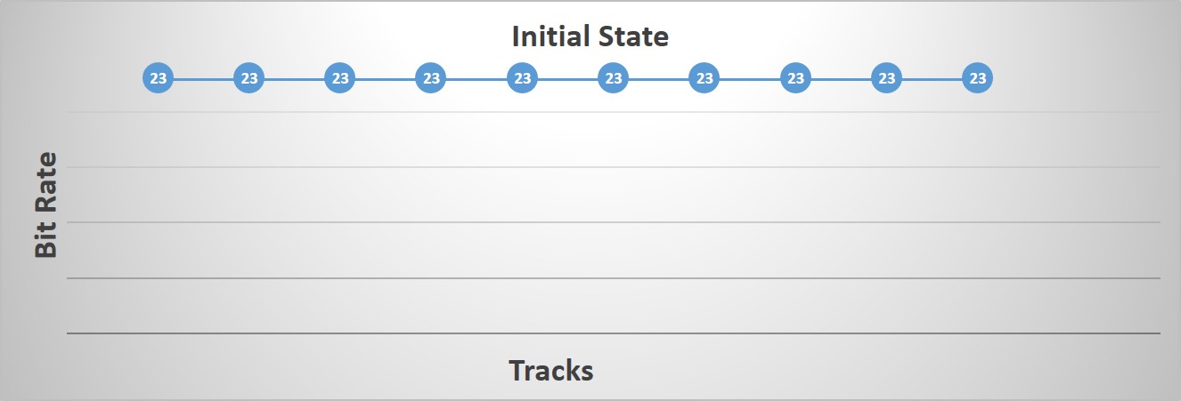
Initial State
In order to start our algorithm, we first initialize all our tracks to use the highest bit rate possible. The goal of the algorithm being to lower these values as much as possible while remaining within our accuracy threshold.

First Phase
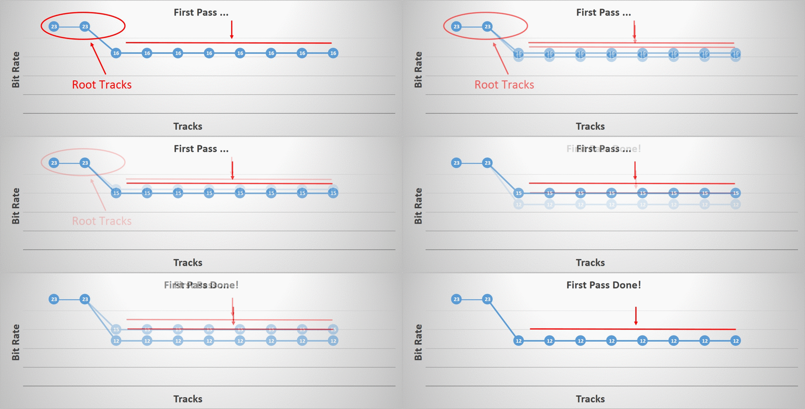
The first phase will lower the bit rate of every track in lock step as much as possible until we cannot do so without exceeding our error threshold. This allows us to quickly trim the search space by finding the best bit rate globally for a given block. However, there is one exception, during the duration of the first phase, the root tracks remain locked to the highest bit rate and thus the highest accuracy. This is done because some clips, such as a world space cinematic, have an unusually high accuracy requirement on the root tracks and if we process them as we do the others, they will negatively bias the rest of the tracks.

Second Phase
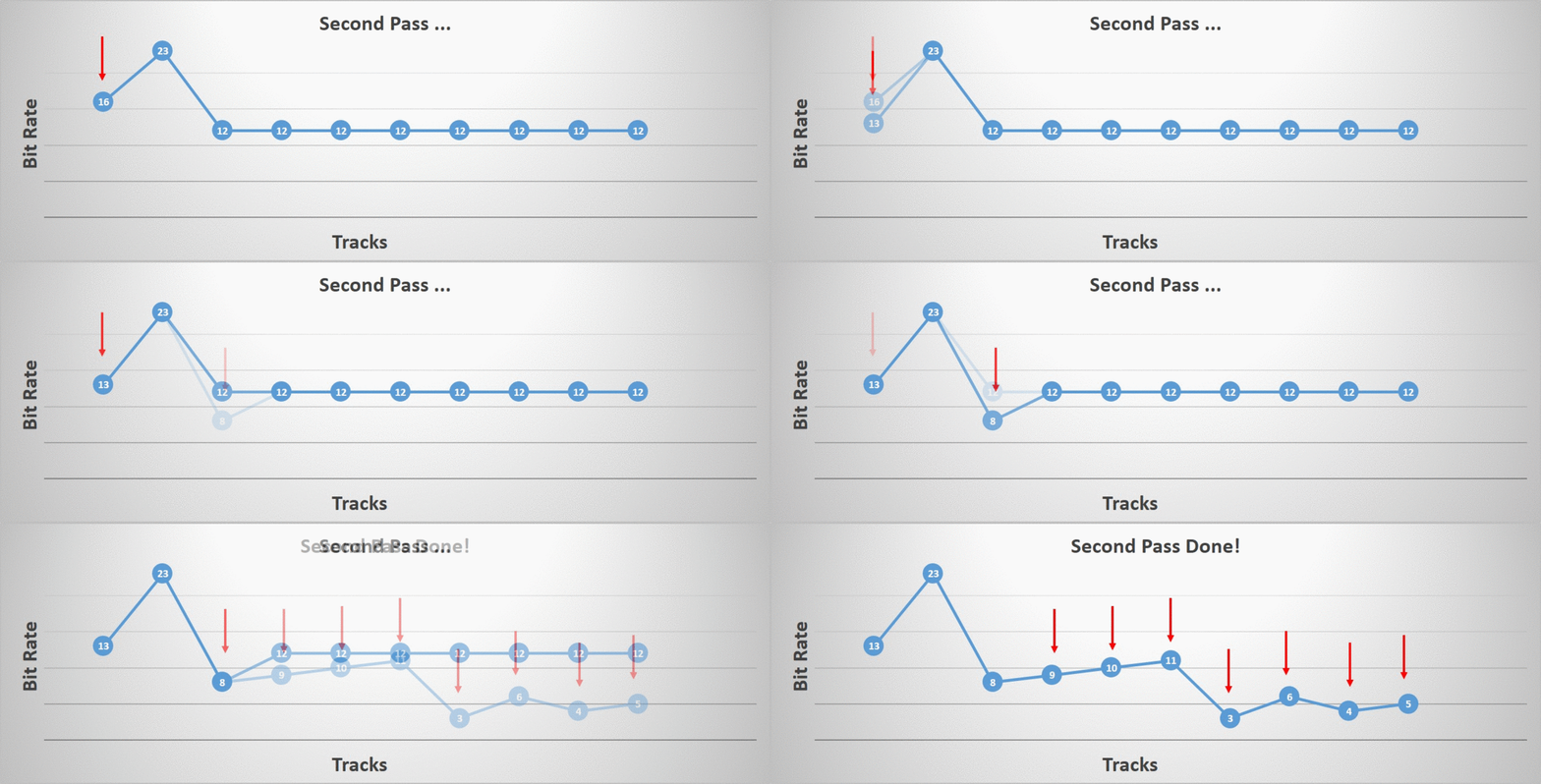
The second phase iterates over all of our tracks and aims to individually lower their bit rate as much as possible up until we reach our error threshold. The algorithm terminates once all tracks have been processed.

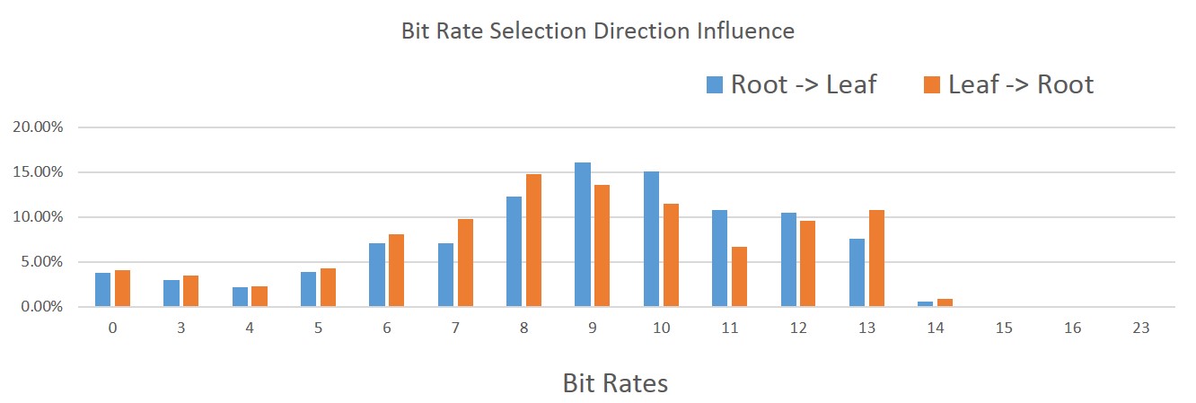
The order in which the tracks are processed matters. I tried two different orderings: starting at the root bone and going down the hierarchy towards the children and the opposite ordering, starting at the leaf bones and going back up towards the root. As it turns out, the distribution of which bit rate was selected by our algorithm changed quite a bit. Note that in the image, the right-most bit rates are very uncommon but they do happen (they are too rare to show up).

Starting at the leaf bones, a higher incidence of lower bit rates were selected. This intuitively makes sense since we have more children than we have parents in our hierarchy. On the other hand, we also have a higher incidence of higher bit rates. Again this makes sense since by lowering the children first, we force the parents to retain more bits in order to preserve the accuracy.
Overall, in the data that I had on hand, starting at the leaf bones and going towards the root resulted in a memory footprint that was roughly 2% smaller without impacting the compression time, accuracy, and our decompression time.
Performance
The compression speed remains acceptable and it can easily be optimized by evaluating all blocks to compress in parallel.
On the decompression side, everything we do is very simple and fast. Since our data is uniform, all of our data is linearly contiguous in memory and a full key frame typically fits within a handful of cache lines (2-5). This is extremely dense and contributes to our very fast decompression. Sadly due to our variable bit rates, we can easily end up performing unaligned reads but their performance remains entirely acceptable on x64 and even with SSE. In fact, with minimal work, everything can be done in SSE and we could even use the streaming read (non-temporal read) intrinsics if we wanted to.